3D-grapher at math3d.org

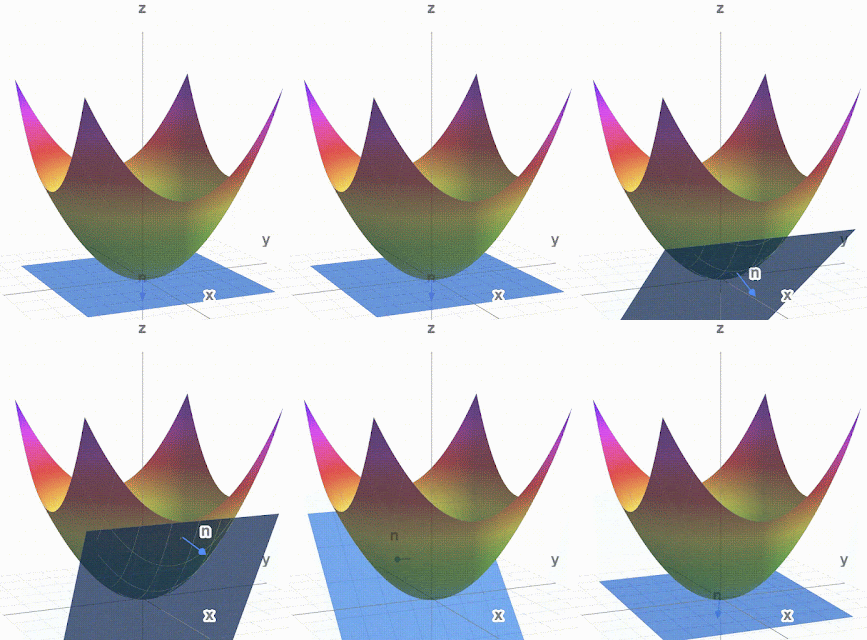
I was practicing my tensor analysis and calculated a normal vector to a surface. I wanted to see it looked orthogonal to the surface. It didn't really. So I made a tangent plane to the surface. The normal vector still looks a bit un-orthogonal but it passes all the mathematical tests.

Paraboloid, Normal vector and tangent plane ##\phi_2\left(\vec{x}\right)=\left(x^1\right)^2+\left(x^2\right)^2-x^3=0##

You can play with this at https://www.math3d.org/ybhLm7KGb and stop it from moving.

I also used Debut Video Capture to make a .avi from math3d and then cloudconvert.com to make the .gif. It is simpler than ezgif.com.

Other surfaces and vectors:

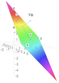
Plane and normal vectors (not v)
Play at https://www.math3d.org/fq5CtGqYa
##\phi_1\left(\vec{x}\right)=x^1+x^2+x^3=5## 

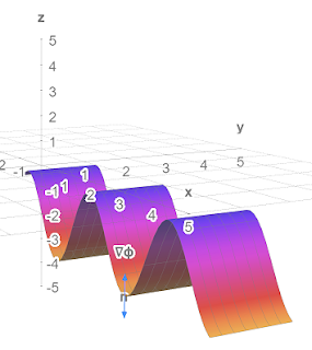
Sine wave with normal vectors
Play at https://www.math3d.org/D8xf0gZMT
##\phi_3\left(\vec{x}\right)=x^3+r_0\cos{\left(kx^1\right)}=-4## 

Lots more tools on Physics Forums at 

List of Online Calculators for Math, Physics, Earth and Other Curiosities.

Cubic equations and elliptic curves

At what ##c## does the curve change from one type to the other and what then is the leftmost point of the curve?

Answers$$c=\sqrt{\frac{32}{27}}\ \ ,\ \ x=-\sqrt{\frac{8}{3}}$$Here's why PF Challenge 2110#14.pdf (7 pages).

A Killing Tensor in FLRW spacetime

God (or the universe) was playing tricks on me last week. In section 8.5 we are looking at redshifts and distances. The latter are more complicated than you might thing. 

I have got to the end of the first paragraph in this section and ignited a controversy on Physics Forums about ##a## the scale factor which tells you how much the universe is expanding. The question is: Is the scale factor a scalar?

We start in an FLRW universe with metric$$
{ds}^2=-{dt}^2+a^2\left(t\right)\left[\frac{{\rm dr}^2}{1-\kappa r^2}+r^2{d\theta}^2+r^2\sin^2{\theta}{d\phi}^2\right]
$$First Carroll invents a tensor$$
K_{\mu\nu}=a^2\left(g_{\mu\nu}+U_\mu U_\nu\right)
$$where ##U^\mu=\left(1,0,0,0\right)## is the 4-velocity of (all) comoving observers. Carroll says it satisfies $$
\nabla_{(\sigma}K_{\mu\nu)}=0
$$"as you can check" and therefore it is a Killing tensor. I accepted the challenge and it took me a few days.

I was not sure if the scale factor ##a## is a scalar. If it's not then it is doubtful whether ##K_{\mu\nu}## is even a tensor. If ##a## is not a scalar but somehow ##K_{\mu\nu}## is a tensor then we must calculate ##\nabla_\sigma K_{\mu\nu}## by expanding the covariant derivative:$$
\nabla_\sigma K_{\mu\nu}=\mathrm{\partial}_\sigma K_{\mu\nu}-\Gamma_{\sigma\mu}^\lambda K_{\lambda\nu}-\Gamma_{\sigma\nu}^\lambda K_{\mu\lambda}
$$If ##a## is a scalar then we can use the Leibniz rule: $$
\nabla_\sigma K_{\mu\nu}=\left(g_{\mu\nu}+U_\mu U_\nu\right)\nabla_\sigma\left(a^2\right)+a^2\nabla_\sigma\left(g_{\mu\nu}+U_\mu U_\nu\right)
$$I used Leibniz first and failed. Then I was inspired by a simpler version on physics.stackexchange and got the right answer using the first formula. That made me doubt that ##a## was a scalar. So I asked about it on Physics Forums. Then I found my error in the Leibniz method and it gave the right answer! So now I think that ##a## is a scalar after all. The Leibniz way is a good deal more efficient than the first.  The discussion continues and I think that PeterDonis has had the last word although vanhees71 is still wriggling at ##11. He surrenders at #13.

Read it all at Commentary 8.5 Killing Tensor in FLRW spacetime.pdf. (7 pages)

Inverses, determinants, Levi-Civita symbol and Laplacian

I have been wandering among inverses of matrices and tensors, determinants, Levi-Civita symbol and the Laplacian and found a wonderful formula for an inverse tensor (4). This leads to the differential equation connecting the determinant of a tensor, the determinant of its inverse, its inverse and itself at (5) and (6). The former can be used to prove the equivalence of Wikipedia's (7) Carroll's (8) formulas for the Laplacian which was where this all started.

I have presented the chain of reasoning as a set of questions and answers:

Questions

Consider the following:

For a square matrix ##A## and its inverse ##A^{-1}##
\begin{align}
A^{-1}=\frac{1}{\det{\left(A\right)}}adj{\left(A\right)}&\phantom {10000}(1)\nonumber
\end{align}The adjugate is the transpose of the cofactor matrix. The cofactor matrix is the matrix whose ##i,j##th element is the ##\left(-1\right)^{i+j}## times the determinant of the matrix formed by removing row ##i## column ##j## from ##A##.

a) Prove that equation (1) is true. Easy.

b) Rewrite it in component form. Very easy.

Carroll's 2.66 for the determinant of a matrix ##A## with components ##A_{\ \ \ \ \ {\mu\prime}_1}^{\mu_1}##, was

\begin{align}{\widetilde{\epsilon}}_{{\mu\prime}_1{\mu\prime}_2\ldots{\mu\prime}_n}\det{\left(A\right)}={\widetilde{\epsilon}}_{\mu_1\mu_2\ldots\mu_n}A_{\ \ \ \ \ {\mu\prime}_1}^{\mu_1}A_{\ \ \ \ \ {\mu\prime}_2}^{\mu_2}\ldots A_{\ \ \ \ \ {\mu\prime}_n}^{\mu_n}&\phantom {10000}(2)\nonumber
\end{align}Vanhees71's PF post uses the first simplification of (2) in four dimensions and then says, slightly rearranged, that components of ##g^{\mu_11}## are

\begin{align}
gg^{\mu_11}=\left(-1\right)^{\mu_1}\epsilon^{\mu_1\mu_2\mu_3\mu_4}g_{\mu_22}g_{\mu_33}g_{\mu_44}&\phantom {10000}(3)\nonumber
\end{align}I find a more general formula 

\begin{align}
\left|A\right|{\bar{A}}^{\alpha\mu_\alpha}=\epsilon^{\mu_1\mu_2\mu_3\ldots\mu_n}\prod_{\beta\neq\alpha} A_{\mu_\beta\beta}&\phantom {10000}(4)\nonumber
\end{align}Vanhees71 used (3) to get

\begin{align}
\partial_\nu g=gg^{\rho\sigma}\partial_\nu g_{\rho\sigma}&\phantom {10000}(5)\nonumber
\end{align}c) Are (3) and (4) (in 4 dimensions) the same? Easy.

d) Use (2) to prove that the correct one really is correct. Hard.

e) Use the correct one to prove (5). Middling.

f) Prove the generalization of (5):

\begin{align}
\left|\bar{A}\right|\partial_\nu\left|A\right|={\bar{A}}^{\rho\sigma}\partial_\nu A_{\sigma\rho}&\phantom {10000}(6)\nonumber
\end{align}There is a Wikipedia formula in "arbitrary curvilinear coordinates in N dimensions" for the Laplacian:

\begin{align}
\nabla^2=\frac{1}{\sqrt{\left|g\right|}}\frac{\partial}{\partial x^i}\left(\sqrt{\left|g\right|}g^{ij}\frac{\partial}{\partial x^j}\right)&\phantom {10000}(7)\nonumber
\end{align}And Carroll's formula (from exercise 3.4):

\begin{align}
\nabla^2=\nabla_\mu\nabla^\mu=g^{\mu\nu}\nabla_\mu\nabla_\nu&\phantom {10000}(8)\nonumber
\end{align}g) Use (5) to prove that (7) and (8) are the same. Middling to hard.

Answers

c) No, d) The correct one is (4). The rest of the answers are in the first six pages of 

Commentary 2.8 Inverses Levi-Civita and more.pdf 

The remaining six pages contain examples to test the answers and check progress.

Robertson-Walker metrics

In section 8.2 we meet what Carroll calls the Robertson-Walker metrics:$$
{ds}^2=-{dt}^2+R^2\left(t\right)\left[\frac{{d\bar{r}}^2}{1-k{\bar{r}}^2}+{\bar{r}}^2{d\Omega}^2\right]=-{dt}^2+a^2\left(t\right)\left[\frac{{\rm dr}^2}{1-\kappa r^2}+r^2{d\Omega}^2\right]
$$The second version is Carroll's preferred form - 'flouting' conventional wisdom.

Four people found the equations in various teams. They are Alexander Friedmann (Russian), Georges Lemaître (Belgian), Howard Robertson (USian) and Arthur Walker (British) and the metrics are often named after one or some or all. Carroll favours the English speakers.

As usual I check Carroll's equations and (not so usual) have three minor complaints.

1) When he gives the Christoffel symbols at his equation 8.44 the third line is$$
\Gamma_{01}^1=\Gamma_{02}^2\ \ \ \ \ \ \ \ \ \ \ \ \ \ \ \ \ \Gamma_{03}^3=\frac{\dot{a}}{a}
$$there should be an ##=## sign between ##\Gamma_{02}^2## and ##\Gamma_{03}^3##!

2) Just after equation 8.35 he says that a flat 3-manifold could be described by 'a more complicated manifold such as the three-torus ##S^1\times S^1\times S^1##'. How can a torus, something generated by circles, be flat? I think he should have said a flat thee-torus. It can be generate from three circles but not as simply as the usual doughnut which is not flat.

3) Before that, just after equation 8.29, he says ##k## sets the curvature and therefore the size of the spatial surfaces. One might think that ##k=0## sets the size as infinite (flat curvature) but the aforementioned flat three-torus is a counter example with ##k=0## and finite size. So ##k=0## does not set the size as you might have expected. Similar arguments apply when ##k<0##.

I learned a few other things too: I suspected that if the metric is diagonal then the Ricci tensor must be diagonal. Not true! But on the plus side I found Win's supercharged formula for calculating Ricci tensor components in that case. It avoids the need to calculate Christoffel and Riemann components. I also learned a bit more about smooth isometric embedding.

I also noticed something slightly mysterious that Carroll does not draw to our attention: In the closed universe case (finite size?) the radial coordinate ##\bar{r}## is constrained by ##{\bar{r}}^2<1##. So the universe might be even more closed than we thought.

Read it all at Commentary 8.2 Robertson-Walker Metrics.pdf (7 pages + 5 of calculations)

 

Curvature of a torus

Torus from Wikipedia

Carroll seems to say that a three-torus can have curvature zero everywhere. A two-torus does not. 

It has a curvature ##S## $$S=\frac{2\cos{\theta}}{r\left(R+r\cos{\theta}\right)}$$where ##r,R,\theta## are shown on my wire diagram. 

So the curvature is not constant. So a torus is not maximally symmetric. The curvature vanishes at the top and bottom of the torus, is negative on the inside and positive on the outside which is exactly what you would expect. Note that it gets more negative than it gets positive - probably because the inside is closer to the centre and therefore has to curve harder. If ##R=20## the minima and maxima are almost equally far from zero. 

Wrong!

I asked for help on Physics Forums here and you can have a flat torus as shown in the diagram on the right. It is is like a rectangle size ##A\times B## with coordinates ##x,y## but if you go off an edge, you come back to the opposite edge, so adding multiples of ##A## to the ##x## coordinate of ##B## to the ##y## coordinate also keep you in the same place. Pretty similar to the regular torus where adding ##2\pi## to ##\theta## or ##\phi## does the same. The only trick is that you have to start with two circles in four dimensions not three! So Carroll was messing about in six dimensions.

Here's why Commentary 8.2 Tori.pdf. (4 pages).

Curvature in two dimensions

Here we calculate formulas for curvature in two dimensions. Specifically we give coordinates, metrics, Christoffel symbols, Riemann tensors (only twice) and scalar curvature (or Ricci scalar) for ellipsoids, elliptic paraboloids and hyperbolic paraboloids.

Images from Wikipedia: Ellipsoid , Paraboloid

We also find a general formula for the scalar curvature in two dimensions which only requires one component of the Riemann tensor. On the way we find the formulas to calculate all the other non zero Riemann components from the one. With coordinates ##\left(\theta,\phi\right)## which are naturally used for the ellipsoid, the formula for the scalar curvature is $$
R=\frac{2}{g_{\phi\phi}}\left(\partial_\theta\Gamma_{\phi\phi}^\theta-\partial_\phi\Gamma_{\theta\phi}^\theta+\Gamma_{\theta\theta}^\theta\Gamma_{\phi\phi}^\theta+\Gamma_{\theta\phi}^\theta\Gamma_{\phi\phi}^\phi-\Gamma_{\phi\theta}^\theta\Gamma_{\theta\phi}^\theta-\Gamma_{\phi\phi}^\theta\Gamma_{\theta\phi}^\phi\right)
$$This is very similar to the formula given at the very end of the Wikipedia article on Gaussian curvature ##K## which is$$
K=-\frac{1}{E}\left(\frac{\partial}{\partial u}\Gamma_{12}^2-\frac{\partial}{\partial v}\Gamma_{11}^2+\Gamma_{12}^1\Gamma_{11}^2-\Gamma_{11}^1\Gamma_{12}^2+\Gamma_{12}^2\Gamma_{12}^2-\Gamma_{11}^2\Gamma_{22}^2\right)
$$The article also reveals that the scalar curvature is twice the Gaussian curvature. The Wikipedia formula might be better written with all the one indices replaced by ##u## and all the 2 indices replaced by ##v##. Then reverting to ##\theta,\phi## as indices, the thing in brackets in the first formula is ##R_{\ \ \ \phi\theta\phi}^\theta## and in the second is ##R_{\ \ \ \theta\theta\phi}^\phi##. The relationship mentioned above between Riemann components is
\begin{align}
R_{\ \ \ \theta\theta\phi}^\theta&=\frac{g_{\theta\phi}}{g_{\phi\phi}}R_{\ \ \ \phi\theta\phi}^\theta&\phantom {10000}\nonumber\\
R_{\ \ \ \theta\phi\theta}^\theta&=-\frac{g_{\theta\phi}}{g_{\phi\phi}}R_{\ \ \ \phi\theta\phi}^\theta&\phantom {10000}\nonumber\\
R_{\ \ \ \phi\theta\phi}^\theta&=\partial_\theta\Gamma_{\phi\phi}^\theta-\partial_\phi\Gamma_{\theta\phi}^\theta+\Gamma_{\theta\theta}^\theta\Gamma_{\phi\phi}^\theta+\Gamma_{\theta\phi}^\theta\Gamma_{\phi\phi}^\phi-\Gamma_{\phi\theta}^\theta\Gamma_{\theta\phi}^\theta-\Gamma_{\phi\phi}^\theta\Gamma_{\theta\phi}^\phi&\phantom {10000}\nonumber\\
R_{\ \ \ \phi\phi\theta}^\theta&=-R_{\ \ \ \phi\theta\phi}^\theta&\phantom {10000}\nonumber\\
R_{\ \ \ \theta\theta\phi}^\phi&=-\frac{g_{\theta\theta}}{g_{\phi\phi}}R_{\ \ \ \phi\theta\phi}^\theta&\phantom {10000}\nonumber\\
R_{\ \ \ \theta\phi\theta}^\phi&=\frac{g_{\theta\theta}}{g_{\phi\phi}}R_{\ \ \ \phi\theta\phi}^\theta&\phantom {10000}\nonumber\\
R_{\ \ \ \phi\theta\phi}^\phi&=-\frac{g_{\theta\phi}}{g_{\phi\phi}}R_{\ \ \ \phi\theta\phi}^\theta&\phantom {10000}\nonumber\\
R_{\ \ \ \phi\phi\theta}^\phi&=\frac{g_{\theta\phi}}{g_{\phi\phi}}R_{\ \ \ \phi\theta\phi}^\theta&\phantom {10000}\nonumber
\end{align}So now it is easy to work out that the mysterious ##E## in the Wikipedia formula should be ##g_{\theta\theta}## which is the same as ##g_{11}##. 

For the record the scalar curvatures for the ellipsoids, elliptic paraboloids and hyperbolic paraboloids are respectively$$
R_{El}=\frac{2b^2}{\left(a^2\cos^2{\theta}+b^2\sin^2{\theta}\right)^2}
$$$$
R_{Ep}=\frac{2a^2}{\left(1+a^2r^2\right)^2}
$$$$
R_{Hp}=\frac{-8}{\left|g\right|^2a^2b^2}
$$These are a bit vague until you know what the coordinate systems are but you can see what the sign of the curvature is which is what I was interested in.

Why did I do all this?

This was quite a project. It was sparked off by the following:
On Physics Forums Ibix said:
I don't know where you [JoeyJoystick] are getting numbers for the mass of the universe from - our current understanding is that it's infinite in size and mass.
I said:
Universe infinite in size and mass? That's extraordinary. Where can I read more about it, please?
Ibix said:
I would think Carroll covers it - chapter 8 of his lecture notes certainly does. The flat and negative curvature FLRW metrics are infinite in extent and have finite density matter everywhere. Modern cosmological models are a bit more complicated, but retain those features.

Chapter 8 in the book is on Cosmology and about 50 pages long. Part 8 of the lecture notes is on Cosmology and contain 15 pages. I think those are the places to look, but after a quick look I did not find anything specifically about the size of the Universe.

If the universe has flat or negative curvature locally and then we presume that applies everywhere, that implies it is infinite in extent. Presumably shortly after the big bang the universe was finite in extent, so at some time it must have changed from finite to infinite! Maybe that's inflation?

So I decided to test the flatness idea in two dimensions....
Summary in Commentary 8 Curvatures 2D.pdf (6 pages), mostly pictures.
Full details in
Commentary 8 Curvatures 2D calculations.docx
or Commentary 8 Curvatures 2D calculations.pdf (24 pages)

Coordinates and basis vectors

I was still not really sure what is meant by the statement that partials form a coordinate basis. Then if they do, is their character (null, timelike or spacelike) related to the metric? At last I asked on Physics forums and PeterDonis had the final word. So now I do know what is meant by partials forming a coordinate basis and there is some relationship to the metric.

Carroll writes$$
\frac{d}{d\lambda}=\frac{dx^\mu}{d\lambda}\partial_\mu
$$"Thus the partials ##\left\{\partial_\mu\right\}## do indeed represent a good basis for the vector space of the directional derivatives, which we can therefore safely identify with the tangent space."

We have a parabola parameterized by ##\lambda## given by$$t=\frac{\lambda^2}{10}\ ,\ \ x=\lambda$$so$$\frac{dt}{d\lambda}=\frac{\lambda}{5}\ \ ,\ \ \ \frac{dx}{d\lambda}=1$$and the tangent vector ##V=d/d\lambda## has components ##\left(dt / d\lambda , dx/ d \lambda\right)## at ##\left(t,x\right)##.

In plane polar coordinates ##\left(r,\theta\right)## the ##\partial_\theta## basis vector is along lines with parameters ##\left(k_r,\lambda\right)##. So the ##\theta## basis vectors lie on concentric circles around the origin. Similarly ##r## basis vectors are radial.

All you need for plane polar coordinates is a line segment to measure ##\theta## from and one end to serve as the origin. The line is normally drawn horizontally. That is not essential.

See how it all hangs together: Commentary 2.3 Coordinates and basis vectors.pdf 

And the thread on physics forums here.

Proper acceleration, Spaghettification and G2

After that Exercise 5.5 I thought I was an expert on falling into a black hole and and that I could calculate the 'proper acceleration' and spaghettification which is the term used for what happens when acceleration differs so much in different parts of your body that you get stretched out like the doomed lady on the right.

Then there is there is the matter of the gas cloud known as G2, which was discovered heading towards Sagittarius A*, the black hole at the centre of our galaxy, in 2011 by some folk at the Max Planck Institute. G2 was destined to come closest to Sagittarius A* in Spring 2014 "with a predicted closest approach of only 3000 times the radius of the event horizon". There was great excitement because spaghettification and great fireworks were expected. However nothing much happened and G2 continues on its way, orbiting Sagittarius A*.

I attempted to do some calculations and tested them on Physics Forums and got adverse comments from PeterDonis. Ibix was more positive "I think your maths is correct ...". PeterDonis showed me the 'correct' way of calculating proper acceleration and then dragged me back to the geodesic deviation equation which is the right way to calculate spaghettification. But I still don't fully understand said equation and how to use it😭. I also learnt a bit more about units: 'natural' and 'geometric'. PeterDonis is a hard task master.

The correct way to calculate proper acceleration gives infinite acceleration at the event horizon. One benefit of that is that it tells you that you cannot escape falling through it, once close enough. That is true. The drawback is that it makes the radial change in acceleration also infinite. So you will get ripped up at the event horizon. That is not true given a big enough black hole.

Here are my calculations (about four pages) and what I learnt (another three).
Commentary 5.6#4 Proper acceleration.pdf 

Exercise 5.5 Observer and beacon outside black hole

Question

Consider a comoving observer sitting at constant spatial coordinates ##\left(r_\ast\ ,\theta_\ast\ ,\ \phi_\ast\right)## around a Schwarzschild black hole of mass ##M##. The observer drops a beacon onto the black hole (straight down along a radial trajectory). The beacon emits radiation at a constant wavelength ##\lambda_{em}## (in the beacon rest frame).

a) Calculate the coordinate speed of the beacon as a function of ##r##.
b) Calculate the proper speed of the beacon. That is, imagine there is a comoving observer at fixed ##r##, with a locally inertial coordinate system set up as the beacon passes by, and calculate the speed as measured by the comoving observer. What is it at ##r=2GM##?
c) Calculate the wavelength ##\lambda_{obs}##, measured by the observer at ##r_\ast##, as a function of the radius ##r_{em}## at which the radiation was emitted.
d) Calculate the time ##t_{obs}## at which a beam emitted by the beacon at radius ##r_{em}## will be observed at ##r_\ast##.
e) Show that at late times, the redshift grows exponentially: ##\lambda_{obs}/\lambda_{em}\propto e^{t_{obs}/T}##. Give an expression for the time constant ##T## in terms of the black hole mass ##M##.

Answers

This question is a fascinating can of worms. I needed the help of an unwitting mentor Jeriek Van den Abeele from the University of Oslo. The first crucial help was to use the timelike killing vector constant $$
E=\left(1-\frac{2GM}{r}\right)\frac{dt}{d\tau}
$$This came in useful not only for the beacon velocities but also for the  travel time of the photon back to the observer at ##\ r_\ast## in question d.

I also needed help from Physics Forums on comoving coordinates and I think I understand them now, although there was some dispute about how the (second)  comoving observer in question (b) would actually achieve that state. When people talk about comoving coordinates for the Universe, they are talking about something quite different from here: Coordinates comoving with the Universe are growing with the Universe.

Part of the worminess arises from confusion about what coordinates are referring to what. There was a profusion of subscripts: ##r_{em},r_\ast,\ R_s,t_\gamma,t_{em},t_{obs},t_b##. The last of those was introduced gratuitously by my mentor who I refer to as Oslo. In my opinion ##t_b\equiv t_{em},\ \ r_b\equiv r_{em}##. I try to avoid these subscripts as much as possible.

I got two answers to question (b). One was the proper speed calculated in the strange comoving inertial coordinate system, as Carroll asked, and the other was the proper speed in Schwarzschild coordinates. I called them ##dr^\prime/d\tau^\prime## and ##dr/d\tau##. The first was what Carroll asked for and can be used (but is not essential) in question (c). Apart from that I am not sure how useful it is. ##dr/d\tau## is what would be experienced by an astronaut falling with the beacon and it does not reach the speed of light at the event horizon.

Interestingly I calculated the answer to (c) using Doppler redshift + gravitational redshift and Oslo did it in one leap - which was more complex and contained a small error which had no effect. The formulas in the two answers looked quite different but when plotted gave the same lines. Eventually I proved that the formulas were in fact the same.

As usual the actual geodesic equations are not used to find out about all these geodesics. Nevertheless I will have a try to see if I can do better with that beacon in section 5.6.

Read it all at Ex 5.5 Observer and beacon.pdf (11 pages not including other documents)

Lagrange Formulation of General Relativity

Section 4.3 on the Lagrange formulation of General Relativity was pretty tough. I had to start by reading and understanding section 1.10 on classical field theories of which I knew nothing. That took about a month. Back on this section  I got very confused about small variations, which are vital for this branch of calculus. I was misled (even lied to) by JG on math.stackexchange and then helped by Physics Forums. I had to collect all my new knowledge about variations in a separate commentary. Carroll threw several interesting  challenges at me. We end with a new definition of the energy momentum tensor.

Read my thoughts: Commentary 4.3 Lagrange Formulation of GR.pdf (7 pages)
And nuggets on variations: Commentary Variations of objects as in calculus of variations.pdf (3 pages)

Planck dimensions

At equations 4.91-4.95 Carroll gives the Planck's set of four dimensioned quantities: Planck's mass, length, time and energy. I wanted to compare them with actual things. Planck first noticed these way back in 1899.
\begin{align}

m_p=\sqrt{\frac{\hbar c}{G}}&=2.18\times{10}^{-8}\rm{kg}&\rm{{10}^{7}\ E. coli}\phantom {100000000000000000000}&\phantom {10000}(1)\nonumber\\

l_p=\sqrt{\frac{\hbar G}{c^3}}&=1.63\times{10}^{-35}\rm{m}&\rm{Radius\ of\ proton\ ={10}^{-15}\ m}\phantom {10000}&\phantom {10000}(2)\nonumber\\

t_p=\sqrt{\frac{\hbar G}{c^5}}&=5.39\times{10}^{-44}\rm{s}&\rm{Cosmic\ inflation\ ends\ at\ {10}^{-32}s}\phantom {10000}&\phantom {10000}(3)\nonumber\\

E_p=\sqrt{\frac{\hbar c^5}{G}}&=1.95\times{10}^9\rm{J}&\rm{Sun\ emits{\ 10}^{26}\ Js^{-1}.  \text{ A-bomb}\rm={10}^{12}}\ J&\phantom {10000}(4)\nonumber\\

&=1.22\times{10}^{19}\rm{GeV}&

&\phantom {10000}\nonumber

\end{align}

Max Planck 1858-1947

He then says "Most likely, quantum gravity does not become important until we consider particle masses greater than ##m_p##, or times shorter than ##t_p##, or lengths smaller than ##l_p##, or energies greater than ##E_p##; at lower scales classical GR should suffice. Since these are all far removed from observable phenomena, constructing a consistent theory of quantum gravity is more an issue of principle than of practice."

Whilst it is unimaginable that we will see things shorter than ##t_p## or smaller than ##l_p##, particle masses ('point masses') greater than ##m_p## are commonplace in GR and energies greater than ##E_p## are happening all the time. Can anybody help me make sense of the ##m_p,E_p## parts? And why are those 'greater than' and the others 'less than'?

I found out when I asked on physics forums. Read it at Commentary 4.5 Planck dimensions.pdf (2 pages).

The energy-momentum tensor in SR

Fluid flow by Thierry Dugnolle

Many moons ago I had skipped the end of section 9 and all of section 10 in chapter 1. It is time to return to them and flat space time starting with the end of section 9 it looks at the energy-momentum tensor for a perfect fluid. I had written at the top of the page "? don't follow much of this from 1.116". Now I do. It shows how to get from that tensor to two well known classical (non-relativistic) equations in the non-relativistic limit: a continuity equation and the Euler equation from fluid dynamics. This gives us faith that the tensor is correct - even though I had not heard of either of these equations.

Along the way we find some tricks with four-velocity ##U^\mu={dx^\mu} / {d\tau}##, meet the projection tensor ##P_{\ \ \ \ \nu}^\sigma## which projects a vector orthogonal to another do some dimensional analysis and find out what energy density really is (I missed this in the book, or Carroll forgot to mention it). I had to consult the great Physics Forums on that and got liked for a facetious comment about measuring it in £sd 😀- I'm sure that oil companies must do it: kerosene is more valuable per kg than bunker fuel.

All the details here Commentary 1.9 Energy Momentum Tensor.pdf (6 pages)

The Laplacian

Laplace 1749-1827

The second equation in chapter 4 was Poisson's differential equation for the gravitational potential ##\Phi##:
\begin{align}
\nabla^2\Phi=4\pi G\rho&\phantom {10000}(1)\nonumber
\end{align}What does ##\nabla^2## mean? A quick look on the internet reveals that it is the Laplace operator or Laplacian sometimes written ##\Delta## (capital delta) or possibly ##∆## (which Microsoft describes as increment). They come out different in latex \Delta and ∆ respectively. I should use the former.

I have found various formulations for the Laplacian and I want to check that they are all really the same. Two are from Wikipedia and the third is from Carroll. They are:
A Wikipedia formula in ##n## dimensions:
\begin{align}
\nabla^2=\frac{1}{\sqrt{\left|g\right|}}\frac{\partial}{\partial x^i}\left(\sqrt{\left|g\right|}g^{ij}\frac{\partial}{\partial x^j}\right)&\phantom {10000}(2)\nonumber
\end{align}A Wikipedia formula in "in 3 general curvilinear coordinates ##(x^1,x^2,x^3)##":
\begin{align}
\nabla^2=g^{\mu\nu}\left(\frac{\partial^2}{\partial x^\mu\partial x^\nu}-\Gamma_{\mu\nu}^\lambda\frac{\partial}{\partial x^\lambda}\right)&\phantom {10000}(3)\nonumber
\end{align}And Carroll's formula (from exercise 3.4) which I did not understand at the time because I had not spotted the second step:
\begin{align}
\nabla^2=\nabla_\mu\nabla^\mu=g^{\mu\nu}\nabla_\mu\nabla_\nu&\phantom {10000}(4)\nonumber
\end{align}The Wikipedia also gives a formula for the Laplacian in spherical polar coordinates:
\begin{align}
\nabla^2f&=\frac{1}{r^2}\frac{\partial}{\partial r}\left(r^2\frac{\partial f}{\partial r}\right)+\frac{1}{r^2\sin{\theta}}\frac{\partial}{\partial\theta}\left(\sin{\theta}\frac{\partial f}{\partial\theta}\right)+\frac{1}{r^2\sin^2{\theta}}\frac{\partial^2f}{\partial\phi^2}&\phantom {10000}(5)\nonumber\\

&=\frac{1}{r}\frac{\partial^2}{\partial r^2}\left(rf\right)+\frac{1}{r^2\sin{\theta}}\frac{\partial}{\partial\theta}\left(\sin{\theta}\frac{\partial f}{\partial\theta}\right)+\frac{1}{r^2\sin^2{\theta}}\frac{\partial^2f}{\partial\phi^2}&\phantom {10000}(6)\nonumber
\end{align}where ##\phi##  represents the azimuthal angle and ##\theta## the zenith angle or co-latitude. So the metric will be
\begin{align}
g_{\mu\nu}=\left(\begin{matrix}1&0&0\\0&r^2&0\\0&0&r^2\sin^2{\theta}\\\end{matrix}\right)&\phantom {10000}(7)\nonumber
\end{align}I assumed that the coordinates are ordered ##r,\theta,\phi## although Wikipedia does not say that.

I want to prove that
A) (2), (3) and (4) both give (5) or (6) the Laplacian in spherical polar coordinates.
B) (4) is equivalent to (3) the general 3-dimensional expression.
C) (4) is equivalent to (2) the general 𝑛-dimensional expression.
A was quite easy. B follows immediately from the formula for the covariant derivative. But in 2020 I could not prove C. In January 2021 I found and proved the Voss-Weyl formula and C becomes easy.

The proofs are in Commentary 4.1 Laplacian.pdf on the first three pages. The other four record my 2020 struggles.

I spent far too long on this but
1) Revisited using the Levi-Civita symbol for expanding determinant (47)
2) Met the log, exponent, trace of a matrix (63) and for diagonal matrices (67)
3) Used diagonalizing matrices (65)
4) Used the product operator ##\prod\ ##for the first time at (27) and again at (66)
5) Proved that ##\ln{\left(\det{\left(A\right)}\right)}=tr{\left(\ln{\left(A\right)}\right)}## (66)
6) Found a formula for the log of a derivative (73)
7)  Found a formula for the log of a matrix (76)

Thanks to Physics forums with whose I proved C for a diagonal metric but they did not know about Voss-Weyl.

Question on cosmological redshift

I have a question on cosmological redshift which I have just learned about from Sean Carroll. After calculating it for an expanding universe he does a thought experiment to show that it is different to Doppler redshift which would be detected if two galaxies were flying away from each other in a flat (therefore not expanding) universe.

We have flat universe L on the left with two galaxies separated by distance ## s##. A photon is emitted from galaxy 1, galaxy 2 is quickly propelled to a separation of ##2s##, galaxy 2 stops and the photon arrives. Since the galaxies are now not relatively moving there would be no Doppler redshift.

On the right the galaxies are also separated by ## s## but, instead of moving a galaxy, the universe expands by a factor of 2 (it briefly gets a metric like ## ds^2=-dt^2+t^2dx^2##), then stops expanding and then the photon arrives. According to the cosmological redshift formula, the photon has a redshift.

This implies that the galaxies in universe R are still separated by ## s##, because rulers would expand along with everything else. One can also check this by drawing out and back light paths before and after expansion.

This is spooky. It also implies that in our 'expanding' universe distant galaxies are not really moving away! One also wonders how we tell that it's cosmological not Doppler redshift.

Have I got the picture roughly right? The next step will be to compare these to real values like the Hubble constant.
On PP at https://www.physicsforums.com/threads/have-i-got-the-right-picture-for-cosmological-redshift.977816/

The great Orodruin replied:

He wrote about this in January 2018 here. It's about 10 pages and the punch line is:
"This example underlines the main message of this Insight: That the assignment of properties and interpretations based on an assumed set of preferred coordinates is not necessarily coordinate invariant and we need to be careful not to impose any coordinate interpretation as absolute truth. In particular, I have seen many instances where people in popular texts make a very strong claim that cosmological redshift is fundamentally different from Doppler shift. The computations above clearly show that this is not the case, instead cosmological redshift and Doppler shift are two sides of the same coin, just viewed in different coordinates. I also have to admit to being among the set of people who did this error until I actually performed these calculations myself."

I have scanned the article (thus getting to the punch line). It deserves further study, especially I know more about the  Robertson–Walker (RW) universe which are the subject of chapter 8 section 2.

Question about geodesic on sphere

I am working from Sean Carroll's Spacetime and Geometry : An Introduction to General Relativity and have got to the geodesic equation. I wanted to test it on the surface of a sphere where I know that great circles are geodesics and is about the simplest non-trivial case I can think of.

Carroll derives the geodesic equation:
\begin{align}
\frac{d^2x^\sigma}{d\lambda^2}+\Gamma_{\mu\nu}^\sigma\frac{dx^\mu}{d\lambda}\frac{dx^\nu}{d\lambda}=0&\phantom {10000}(1)\nonumber
\end{align}##\Gamma_{\mu\nu}^\sigma## is the Christoffel symbol (torsion-free and metric compatible)
\begin{align}
\Gamma_{\mu\nu}^\sigma=\frac{1}{2}g^{\sigma\rho}\left(\partial_\mu g_{\nu\rho}+\partial_\nu g_{\rho\mu}-\partial_\rho g_{\mu\nu}\right)&\phantom {10000}(2)\nonumber
\end{align}In this case the indices are 0,1 and ##x^0=\phi## the colatitude (angle from north pole), ##\ x^1=\theta## , longitude. The metric and inverse metric are
\begin{align}
g_{\mu\nu}=\left(\begin{matrix}1&0\\0&\sin^2{\phi}\\\end{matrix}\right)\ \ ,\ \ g^{\mu\nu}=\left(\begin{matrix}1&0\\0&\sin^{-2}{\phi}\\\end{matrix}\right)&\phantom {10000}(3)\nonumber
\end{align}Those should give me equations for ## \phi,\theta## parameterized by ## \lambda##.

I now expand the second term in (1) for ## \sigma=1## and using the fact that ## \Gamma## is torsion-free (##\Gamma_{\mu\nu}^\sigma=\Gamma_{\nu\mu}^\sigma##).
\begin{align}
\Gamma_{\mu\nu}^1\frac{dx^\mu}{d\lambda}\frac{dx^\nu}{d\lambda}&=\Gamma_{00}^1\frac{dx^0}{d\lambda}\frac{dx^0}{d\lambda}+2\Gamma_{10}^1\frac{dx^1}{d\lambda}\frac{dx^0}{d\lambda}+\Gamma_{11}^1\frac{dx^1}{d\lambda}\frac{dx^1}{d\lambda}&\phantom {10000}(4)\nonumber\\

&=\Gamma_{00}^1\left(\frac{d\phi}{d\lambda}\right)^2+2\Gamma_{10}^1\frac{d\phi}{d\lambda}\frac{d\theta}{d\lambda}+\Gamma_{11}^1\left(\frac{d\theta}{d\lambda}\right)^2&\phantom {10000}(5)\nonumber
\end{align}using the metric and (2) and taking each ## \Gamma## in turn, many terms vanish because the metric components are constant or 0
\begin{align}
\Gamma_{00}^1&=\frac{1}{2}g^{1\rho}\left(\partial_0g_{0\rho}+\partial_0g_{\rho0}-\partial_\rho g_{00}\right)=g^{1\rho}\partial_0g_{0\rho}&\phantom {10000}(6)\nonumber\\

&=g^{10}\partial_0g_{00}+g^{11}\partial_0g_{01}=0&\phantom {10000}(7)\nonumber\\
2\Gamma_{10}^1&=g^{1\rho}\left(\partial_1g_{0\rho}+\partial_0g_{\rho1}-\partial_\rho g_{10}\right)=g^{1\rho}\partial_1g_{0\rho}+g^{1\rho}\partial_0g_{\rho1}&\phantom {10000}(8)\nonumber\\

&=g^{10}\partial_1g_{00}+g^{11}\partial_1g_{01}+g^{10}\partial_0g_{01}+g^{11}\partial_0g_{11}&\phantom {10000}(9)\nonumber\\

&=\frac{1}{\sin^2{\phi}}\frac{\partial}{\partial\phi}\left(\sin^2{\phi}\right)=\frac{2\sin{\phi}\cos{\phi}}{\sin^2{\phi}}=2\cot{\phi}&\phantom {10000}(10)\nonumber\\
\Gamma_{11}^1&=\frac{1}{2}g^{1\rho}\left(\partial_1g_{1\rho}+\partial_1g_{\rho1}-\partial_\rho g_{11}\right)=g^{1\rho}\partial_1g_{\rho1}-\frac{1}{2}g^{1\rho}\partial_\rho g_{11}&\phantom {10000}(11)\nonumber\\

&=g^{10}\partial_1g_{01}+g^{11}\partial_1g_{11}-\frac{1}{2}g^{10}\partial_0g_{11}-\frac{1}{2}g^{11}\partial_1g_{11}&\phantom {10000}(12)\nonumber\\

&=\frac{1}{2}\frac{1}{\sin^2{\phi}}\frac{\partial}{\partial\theta}\left(\sin^2{\phi}\right)=0&\phantom {10000}(13)\nonumber
\end{align}Putting the expressions for ## \Gamma## back into (5) we get
\begin{align}
\Gamma_{\mu\nu}^1\frac{dx^\mu}{d\lambda}\frac{dx^\nu}{d\lambda}&=2\cot{\phi}\frac{d\phi}{d\lambda}\frac{d\theta}{d\lambda}&\phantom {10000}(14)\nonumber
\end{align}Putting that back into (1) we have
\begin{align}
\frac{d^2\theta}{d\lambda^2}+2\cot{\phi}\frac{d\phi}{d\lambda}\frac{d\theta}{d\lambda}=0&\phantom {10000}(15)\nonumber
\end{align}I can use the same method to get a solution for ## \sigma=0##, but that's not relevant yet. Put together they show that lines of longitude are always geodesics as is the equator. So far so good… but

A great circle equation (which we know is a geodesic) can be written as
\begin{align}
\theta=\lambda\ \ ,\ \ \phi=\tan^{-1}{\left(\frac{C}{A\cos{\lambda}+B\sin{\lambda}}\right)}&\phantom {10000}(16)\nonumber
\end{align}where ## A,B,C## are constants depending on the start and end points. I calculated this and checked it against the slightly ambiguous Wolfram maths article at http://mathworld.wolfram.com/GreatCircle.html.

From (16) clearly
\begin{align}
\frac{d^2\theta}{d\lambda^2}=0&\phantom {10000}(17)\nonumber
\end{align}so the other term in (15) should always be zero. It is
\begin{align}
2\cot{\phi}\frac{d\phi}{d\lambda}\frac{d\theta}{d\lambda}=-2\frac{\left(B\cos{\lambda}-A\sin{\lambda}\right)\left(A\cos{\lambda}+B\sin{\lambda}\right)}{C^2+\left(A\cos{\lambda}+B\sin{\lambda}\right)^2}&\phantom {10000}(18)\nonumber
\end{align}which is not always zero! So something is wrong.
It's either
(15) which I have calculated in another way to check it or
(16) which I have also plotted and gives good results or
my differentiation of ##\frac{d\phi}{d\lambda}## which I checked with Symbolab: https://www.symbolab.com/solver/ordinary-differential-equation-calculator/?or=dym&query=%5Cfrac%7Bd%7D%7Bdx%7D(%5Carctan(%5Cfrac%7BC%7D%7BD%5Ccos(x)%2BB%5Csin(x)%7D))

Help! What has gone wrong?
On Physics Forums at https://www.physicsforums.com/threads/question-about-geodesic-on-sphere.975370/

Question on partial derivative

I am working on the geodesic equation for the surface of a sphere. While doing so I come across the partial derivative
\begin{align}
\frac{\partial}{\partial\theta}\left(\sin^2{\phi}\right)=0?&\phantom {10000}(1)\nonumber
\end{align}where ## \phi, \theta## are colatitude(angle from north pole) and longitude. I could say that the expression must vanish because ## \phi,\theta## are orthogonal. But I know thate ## \phi## is a function ## \theta##  so I could say, using the chain rule twice, that the expression is
\begin{align}
\frac{\partial}{\partial\theta}\left(\sin^2{\phi}\right)=2\sin{\phi}\cos{\phi}\frac{d\phi}{d\theta}?&\phantom {10000}(2)\nonumber
\end{align}The answer might be very obvious and simple. I think the former is correct but would like some confirmation please.

The detailed reasons for the question are given below. They include my fears about the metric.

The geodesic equation is
\begin{align}
\frac{d^2x^\sigma}{d\lambda^2}+\Gamma_{\mu\nu}^\sigma\frac{dx^\mu}{d\lambda}\frac{dx^\nu}{d\lambda}=0&\phantom {10000}(3)\nonumber
\end{align}where ## \Gamma## is the Christoffel symbol (torsion-free and metric compatible), given by
\begin{align}
\Gamma_{\mu\nu}^\sigma=\frac{1}{2}g^{\sigma\rho}\left(\partial_\mu g_{\nu\rho}+\partial_\nu g_{\rho\mu}-\partial_\rho g_{\mu\nu}\right)&\phantom {10000}(4)\nonumber
\end{align}The coordinates are  ##x^0=\phi## and ##\ x^1=\theta## and the metric and inverse metric are
\begin{align}
g_{\mu\nu}=\left(\begin{matrix}1&0\\0&\sin^2{\phi}\\\end{matrix}\right)\ \ ,\ \ g^{\mu\nu}=\left(\begin{matrix}1&0\\0&\sin^{-2}{\phi}\\\end{matrix}\right)&\phantom {10000}(5)\nonumber
\end{align}## \lambda## will parameterise a line which gives the required geodesic. First I derived what these equations mean and I get two second order differential equations involving ## \phi,\theta,\lambda##. I believe these are
\begin{align}
\frac{d^2\phi}{d\lambda^2}-\sin{\phi}\cos{\phi}\left(\frac{d\theta}{d\lambda}\right)^2=0&\phantom {10000}(6)\nonumber
\end{align}and
\begin{align}
\frac{d^2\theta}{d\lambda^2}+2\cot{\phi}\frac{d\phi}{d\lambda}\frac{d\theta}{d\lambda}=0&\phantom {10000}(7)\nonumber
\end{align}There were two ways to work these equations out. Assuming (2) (that ##{\partial f(\phi)}/{\partial\theta}\neq0##) each method gave a different answer for equation (7) unless I made a mistake, which is quite likely.

I have not yet tried to solve these equations, but I know that a geodesic on a sphere is a great circle so I can work out its equation and it can be written
\begin{align}
\theta=\lambda\ \ ,\ \ \phi=\tan^{-1}{\left(\frac{C}{A\cos{\lambda}+B\sin{\lambda}}\right)}&\phantom {10000}(8)\nonumber
\end{align}where ## A,B,C## are constants depending on the start and end points (in quite a complicated way.) It should be simple to check that (8) satisfies (6) and (7). Clearly ## \phi## depends only on ## \theta## and the start and end points, as one would expect. This leads to the original question.

I checked my equation (8) by using my wonderful 3-D plotter. The geodesics look perfect.

I also searched the internet for the equation and found one on Wolfram MathWorld (http://www.mathworld.wolfram.com/GreatCircle.html). It was slightly different from mine and cause me great pain. It is incorrect! Their colatitudes and latitudes are mixed up. I have told them, but there is no response. I also plotted their solution and it gave a rather long route to Peking. Whatever the case ## \phi## depends on ## \theta## and the start and end points.

(8) tells us that
\begin{align}
\frac{d^2\theta}{d\lambda^2}=0&\phantom {10000}(9)\nonumber
\end{align}Which does not sit well with (7). If I had the metric at (5) 'the wrong way round', it would be
\begin{align}
g_{\mu\nu}=\left(\begin{matrix}\sin^2{\phi}&0\\0&1\\\end{matrix}\right)\ \ ,\ \ g^{\mu\nu}=\left(\begin{matrix}\sin^{-2}{\phi}&0\\0&1\\\end{matrix}\right)&\phantom {10000}(10)\nonumber
\end{align}this would have given (9) at (7). However I want to cross one bridge at a time …

Posted on PF at https://www.physicsforums.com/threads/question-on-partial-derivative.975058/

The first three answers satisfy me that$$
\frac{\partial}{\partial\theta}\left(\sin^2{\phi}\right)=0
$$Equation (8) is just the equation of some line on the sphere, in this case a geodesic.

Second order partial derivatives vanish?

At the end of a long proof I came across something in tensor calculus that seems too good to be true. And if something seems too good to be true .....

The something is that a second order partial derivative vanishes if one of the parts in the denominator is in the same reference frame as the numerator. That is for example
\begin{align}
\frac{{\partial }^2x^{\mu }}{\partial x^{\rho }\partial x^{{\mu }^{'}}}=\frac{{\partial }^2x^{\mu }}{\partial x^{{\mu }^{'}}\partial x^{\rho }}=0 & \phantom {10000}(1) \\
\end{align}The equality of the first two parts follows because partial derivatives commute. We have
\begin{align}
\frac{{\partial }^2x^{\mu }}{\partial x^{{\mu }^{'}}\partial x^{\rho }}=\frac{\partial }{\partial x^{{\mu }^{'}}}\left(\frac{\partial x^{\mu }}{\partial x^{\rho }}\right) & \phantom {10000}(2) \\
\end{align}but\begin{align}
\frac{\partial x^{\mu }}{\partial x^{\rho }}={\delta }^{\mu }_{\rho } & \phantom {10000}(3) \\
\end{align}where ##{\delta }^{\mu }_{\rho }## is the Kronecker delta which is a constant. (3) seems very reasonable because when ##\mu \neq \rho ##, ##\partial x^{\mu }## and ##\partial x^{\rho }## are orthogonal so ##{\partial x^{\mu }}/{\partial x^{\rho }}## vanishes and when ##\mu =\rho ##, ##{\partial x^{\mu }}/{\partial x^{\rho }}=1##.

So (2) is the derivative of a constant which always vanishes. QED.

Have I made a very stupid mistake? Or am I stating something everybody knows?

On PF at https://www.physicsforums.com/threads/second-order-partial-derivatives-vanish.968079/
The good stevendaryl pointed out my error and gave a little example that proved$$
\frac{{\partial }^2x^{\mu }}{\partial x^{\rho }\partial x^{{\mu }^{'}}}≠\frac{{\partial }^2x^{\mu }}{\partial x^{{\mu }^{'}}\partial x^{\rho }}
$$Partial derivatives only commute if they are in the the same coordinate system, so this IS true$$
\frac{{\partial }^2x^{\mu }}{\partial x^{\rho }\partial x^{{\nu }}}=\frac{{\partial }^2x^{\mu }}{\partial x^{{\nu }}\partial x^{\rho }}$$Say we had$$
f\left(x,y\right)=x^2{\mathrm{sin} y\ }
$$then$$
\frac{\partial }{\partial x}\left(\frac{\partial }{\partial y}f\right)=\frac{\partial }{\partial x}\left(x^2{\mathrm{cos} y\ }\right)=2x{\mathrm{cos} y\ }
$$and$$
\frac{\partial }{\partial y}\left(\frac{\partial }{\partial x}f\right)=\frac{\partial }{\partial y}\left(2x{\mathrm{sin} y\ }\right)=2x{\mathrm{cos} y\ }$$Say we had
$$x^{\mu }=z$$then $$\frac{\partial }{\partial x}\left(\frac{\partial }{\partial y}z\right)=0$$and
$$\frac{\partial }{\partial y}\left(\frac{\partial }{\partial x}z\right)=0$$Say we had$$x^{\mu }=y
$$then$$
\frac{\partial }{\partial x}\left(\frac{\partial }{\partial y}y\right)=\frac{\partial }{\partial x}\left(1\right)=0$$and$$
\frac{\partial }{\partial y}\left(\frac{\partial }{\partial x}y\right)=\frac{\partial }{\partial y}\left(\frac{\partial }{\partial x}y\right)=0$$

Question on covariant derivatives

I am reading I am reading Spacetime and Geometry : An Introduction to General Relativity -- by Sean M Carroll and have arrived at chapter 3 where he introduces the covariant derivative ##{\mathrm{\nabla }}_{\mu }##. He makes demands on this which are \begin{align}
\mathrm{1.\ Linearity:}\mathrm{\ }\mathrm{\nabla }\left(T+S\right)=\mathrm{\nabla }T+\mathrm{\nabla }S & \phantom {10000}(1) \\
\mathrm{2.\ Leibniz\ rule:}\mathrm{\nabla }\left(T\ \otimes \ \ S\right)=\left(\mathrm{\nabla }T\right)\ \ \otimes \ \ S+T\ \otimes \ \ \left(\mathrm{\nabla }S\right) & \phantom {10000}(2) \\
{\mathrm{3.\ Commutes\ with\ contractions:}\mathrm{\nabla }}_{\mu }\left(T^{\lambda }_{\ \ \ \lambda \rho }\right)={\left(\mathrm{\nabla }T\right)}^{\mathrm{\ \ \ }\lambda}_{\mu \ \ \lambda \rho } & \phantom {10000}(3) \\
{\mathrm{4.\ Reduces\ to\ partial\ derivative\ on\ scalars:}\mathrm{\nabla }}_{\mu }\phi ={\partial }_{\mu }\phi  & \phantom {10000}(4) \\
\end{align}1,2 and 4 seem reasonable but I cannot understand 3 and he does not seem to use it, even though he implies that he does.

The LHS of (3) seems straight forward\begin{align}
{\mathrm{\nabla }}_{\mu }\left(T^{\lambda }_{\ \ \ \lambda \rho }\right) & ={\partial }_{\mu }T^{\lambda }_{\ \ \ \lambda \rho }+{\mathrm{\Gamma }}^{\lambda }_{\mu \kappa }T^{\kappa }_{\ \ \ \lambda \rho }-{\mathrm{\Gamma }}^{\kappa }_{\mu \lambda }T^{\lambda }_{\ \ \ \kappa \rho }-{\mathrm{\Gamma }}^{\kappa }_{\mu \rho }T^{\lambda }_{\ \ \ \lambda k} & \phantom {10000}(5) \\
 & ={\partial }_{\mu }T^{\lambda }_{\ \ \ \lambda \rho }-{\mathrm{\Gamma }}^{\kappa }_{\mu \rho }T^{\lambda }_{\ \ \ \lambda k} & \phantom {10000}(6) \\
\end{align}Which is very like the rule for the covariant derivative of a (0,1) tensor.

I understand that the ##\mathrm{\nabla }T## in (1) and (2) means ##{\mathrm{\nabla }}_{\sigma}T## where ##T## is some tensor. So the RHS of (3) appears to be ##{\left({\mathrm{\nabla }}_{\sigma}T\right)}^{\mathrm{\ \ \ }\lambda}_{\mu \ \ \lambda \rho }## which leaves too many indices on the RHS. Otherwise the RHS is some kind of derivative with one contra- and three co-variant indices. What is that?

Help!
Posted on Physics Forums at https://www.physicsforums.com/threads/question-on-covariant-derivatives.967509/

Exercise 2.08 Exterior derivative and modified Leibniz rule

This exercise started in section 2.9 on which I wrote a seven page commentary before accepting Carroll's challenge to prove the modified Leibniz rule for the exterior derivative.

Carroll introduces differential forms: "A differential p-form is a completely antisymmetric (0,p) tensor. Thus scalars are automatically 0-forms and dual vectors (downstairs index) are one-forms. We also have the 4-form ##{\epsilon }_{\mu \nu \rho \sigma }##, the Levi-Civita tensor." I had a slight problem with 0- and 1-forms but this was resolved on Physics Forums.

First we meet the wedge product:

Given a##\ p##-form ##A## and a ##q##-form ##B## we can form a ##(p+q)##-form known as the wedge product ##A\wedge B## by taking the antisymmetrised tensor product:
$${\left(A\wedge B\right)}_{{\mu }_1\dots {\mu }_{p+q}}=\frac{\left(p+q\right)!}{p!q!}A_{[{\mu }_1\dots {\mu }_p}B_{{\mu }_{p+1}\dots {\mu }_{p+q}]}$$
I prove that the wedge product of an n-dimensional 2-form and 1-form is completely antisymmetric in any number of dimensions n ##\mathrm{\ge}## 2 and therefore a 3-form.

Then we meet the exterior derivative

$${\left(\mathrm{d}A\right)}_{{\mu }_1\dots {\mu }_{p+1}}=\left(p+1\right){\partial }_{[{\mu }_1}A_{{\mu }_2\dots {\mu }_{p+1}]}$$They both involve the ghastly total antisymmetrisation operation [] on indices. It is defined back in his equation (1.80) as

$$T_{[{\mu }_1\dots {\mu }_n]}=\frac{1}{n!}\left(T_{{\mu }_1\dots {\mu }_n}\pm \mathrm{sum\ over\ permutations\ of}\ {\mu }_1\dots {\mu }_n\right)$$

This led on to Exercise 2.08

Question

Verify (2.78): For an exterior derivative of a product of a p-form ω and a q-form η, we have the modified Leibnitz rule:

$$\mathrm{d}\left(\omega \wedge \eta \right)=\left(\mathrm{d}\omega \right)\wedge \eta +{\left(-1\right)}^p\omega \wedge \left(\mathrm{d}\eta \right)$$

Answer 

Here we have the ghastly total antisymmetrisation operation [] again and nested in itself. I had to invent a new notation

$$\sum_{\mp \mathrm{\circlearrowleft }}{A_{{\mu }_1\dots {\mu }_n}}\equiv \left(A_{{\mu }_1\dots {\mu }_n}\pm \mathrm{sum\ over\ permuta}\mathrm{tions\ of}\ {\mu }_1\dots {\mu }_n\ where\ we\ use\ -\ for\ odd\ permutations\ and\ +\ for\ even.\right)$$

because writing the stuff about the permutations every time would be stupid and does not fit on a line. I expanded each term in the question equation and reached expressions like

$$\frac{{\left(-1\right)}^{p\left(q+1\right)}}{\left(q+1\right)!p!q!}\sum_{\mp \mathrm{\circlearrowleft }}{\left(\sum_{\mp \mathrm{\circlearrowleft }}{{\mathrm{\partial }}_{{\mu }_1}{\eta }_{{\mu }_2\dots {\mu }_{q+1}}}\right){\omega }_{{\mu }_{q+2}\dots {\mu }_{p+q+1}}}$$

where you can see the nested expansions explicitly. Each term had a different variant of the nesting so the nesting had to be removed and I proved, for example and avoiding too many subscripts, that

$$\sum_{\mp \mathrm{\circlearrowleft }}{\left(\sum_{\mp \mathrm{\circlearrowleft }}{{\mathrm{\partial }}_a{\eta }_{c_1\dots c_q}}\right){\omega }_{b_1\dots b_p}}\mathrm{=}\left(q+1\right)!{\left(-1\right)}^{q(p+q)}\sum_{\mp \mathrm{\circlearrowleft }}{{\mathrm{\partial }}_a{\omega }_{b_1\dots b_p}{\eta }_{c_1\dots c_q}}$$

factorials cancelled beautifully but I was left with

$${\mathrm{d}\left(\omega \wedge \eta \right)}_{\ }=\left(\mathrm{d}\omega \right)\wedge \eta ={\left(-1\right)}^{\left(q+p\right)}\omega \wedge \left(\mathrm{d}\eta \right)$$

which is not the same as the modified Leibnitz rule, in other words, junk.

I also show that the equation does not work for two 1-forms. In fact I get$$2\mathrm{d}\left(\omega \wedge \eta \right)=\left(\mathrm{d}\omega \right)\wedge \eta +{\left(-1\right)}^p\omega \wedge \left(\mathrm{d}\eta \right)$$which agrees with my wrong answer. I am within spitting distance of the correct proof!  I hope to come back to this problem.

Read the full account
Commentary 2.9 Differential forms.pdf (7 pages)
Ex 2.08 Exterior derivative and modified Leibnitz rule.pdf (8 pages - I have long thought that he was Leibnitz. That is acceptable, but Leibniz is better.)

There is also an answer here from University of California, Santa Barbara (UCSB).
It starts from ##\mathrm{d}\left(\omega \wedge \eta \right)## and uses the ordinary Leibnitz rule to split that in two. It then manipulates the two parts to convert them into the RHS of the question equation. There are some rather 'hand-waving' steps such as the first line of text "We drop the inner set of antisymmetrization brackets in the second line because the terms are antisymmetrized in all of their indices". It works in the opposite direction to what I did.