Showing posts with label Cool Graphics. Show all posts

Monday, 10 January 2022

New Scientist Christmas Puzzle 2021

 
The grid contains 46 x 72 = 3,312 letters. Hidden inside it are the 118 elements in the periodic table, 17 known fundamental particles and 20 amino acids that make up proteins. They are revealed here. TAU and TIN occur about 15 and 31 times respectively. Two TINs come out of row 44, column 30, one going up and left, the other up and right. IRON and MUON occur three times. All other multiple occurrences are necessary if one is to have words such as ERBIUM, TERBIUM, YTTERBIUM. MUON should occur twice, the second time in MUONNEUTRINO.


The original puzzle is here. The spreadsheet and more are here.

Monday, 22 November 2021

3D-grapher at math3d.org

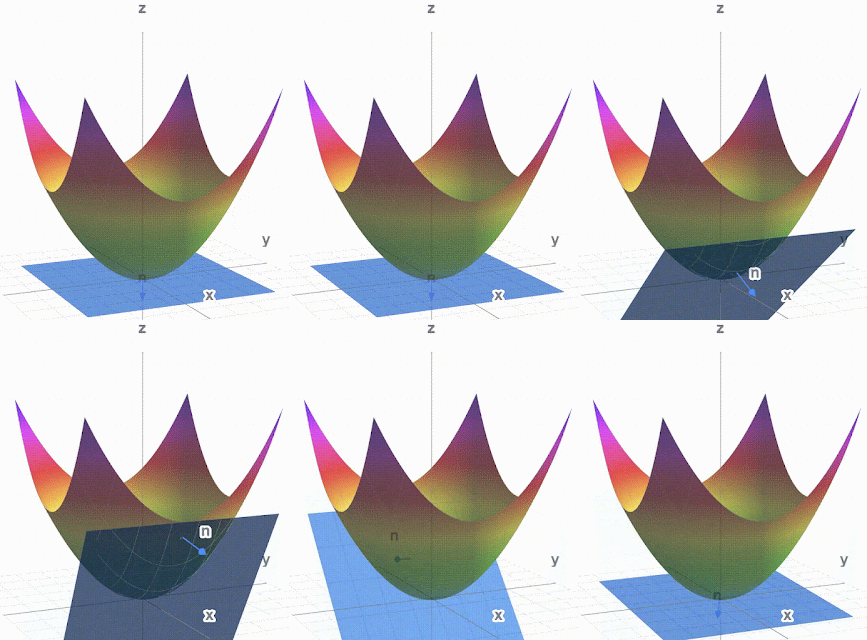
I was practicing my tensor analysis and calculated a normal vector to a surface. I wanted to see it looked orthogonal to the surface. It didn't really. So I made a tangent plane to the surface. The normal vector still looks a bit un-orthogonal but it passes all the mathematical tests.

Paraboloid, Normal vector and tangent plane ##\phi_2\left(\vec{x}\right)=\left(x^1\right)^2+\left(x^2\right)^2-x^3=0##

You can play with this at https://www.math3d.org/ybhLm7KGb and stop it from moving.
I also used Debut Video Capture to make a .avi from math3d and then cloudconvert.com to make the .gif. It is simpler than ezgif.com.

Other surfaces and vectors:
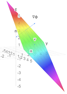
Plane and normal vectors (not v)
Play at https://www.math3d.org/fq5CtGqYa
##\phi_1\left(\vec{x}\right)=x^1+x^2+x^3=5## 


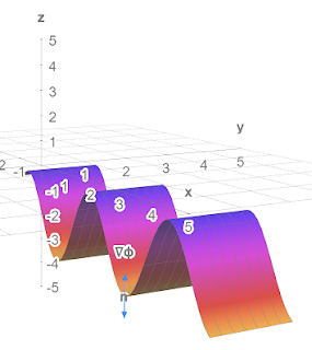
Sine wave with normal vectors
Play at https://www.math3d.org/D8xf0gZMT
##\phi_3\left(\vec{x}\right)=x^3+r_0\cos{\left(kx^1\right)}=-4## 

Lots more tools on Physics Forums at 

Monday, 25 October 2021

Cubic equations and elliptic curves

At what ##c## does the curve change from one type to the other and what then is the leftmost point of the curve?

Answers$$c=\sqrt{\frac{32}{27}}\ \ ,\ \ x=-\sqrt{\frac{8}{3}}$$Here's why PF Challenge 2110#14.pdf (7 pages).

Tuesday, 12 October 2021

The Parallel Propagator and using it on the surface of a sphere

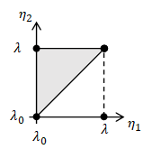
The three page Appendix I is on the parallel propagator which gives a general solution to the parallel transport equation of a vector. The appendix shows how to get this from the parallel transport equation which is, for a vector ##V^\nu## transported along a curve ##x^\mu\left(\lambda\right)## $$\frac{dx^\mu}{d\lambda}\partial_\mu V^\nu+\frac{dx^\mu}{d\lambda}\Gamma_{\mu\sigma}^\nu V^\sigma=0$$First we note that the transported vector can be calculated by$$V^\mu\left(\lambda\right)=P_{\ \ \rho}^\mu\left(\lambda,\lambda_0\right)V^\rho\left(\lambda_0\right)$$where ##V^\rho\left(\lambda_0\right)## is the vector at the start point ##x^\mu\left(\lambda_0\right)## and ##P_{\ \ \rho}^\mu\left(\lambda,\lambda_0\right)## is some matrix which is called the parallel propagator. Next we define another matrix $$A_{\ \ \rho}^\mu\left(\lambda\right)=-\Gamma_{\sigma\rho}^\mu\frac{dx^\sigma}{d\lambda}$$and then show that (dropping indices on the matrices)$$P\left(\lambda,\lambda_0\right)=I+\sum_{n=1}^{n=\infty}T_n$$where ##I## is the identity matrix and $$T_n=\int_{\lambda_0}^{\lambda}{\int_{\lambda_0}^{\eta_n}\int_{\lambda_0}^{\eta_{n-1}}{\ldots\int_{\lambda_0}^{\eta_2}A\left(\eta_n\right)A\left(\eta_{n-1}\right)\ldots A\left(\eta_1\right)}d^n\eta}$$$$=\frac{1}{n!}\int_{\lambda_0}^{\lambda}{\int_{\lambda_0}^{\lambda}\int_{\lambda_0}^{\lambda}{\ldots\int_{\lambda_0}^{\lambda}\mathcal{P}\left[A\left(\eta_n\right)A\left(\eta_{n-1}\right)\ldots A\left(\eta_1\right)\right]}d^n\eta}$$where ##\mathcal{P}## orders the matrices ##A\left(\eta_i\right)## so that ##\eta_n\geq\eta_{n-1}\geq\ldots\geq\eta_1##.
2-simplex

The first integral is over ##n##-dimensional equilateral right triangles, or ##n##-simplices and is quite hard to calculate but ##n!## ##n##-simplices make an ##n##-cube which makes the second integral which is much easier to calculate. I had a bit of trouble getting my head round all that and I tested it on a few examples including vectors transported along lines of constant latitude.  It all works!

Read about it here Commentary App I Parallel Propagator.pdf (13 pages). 

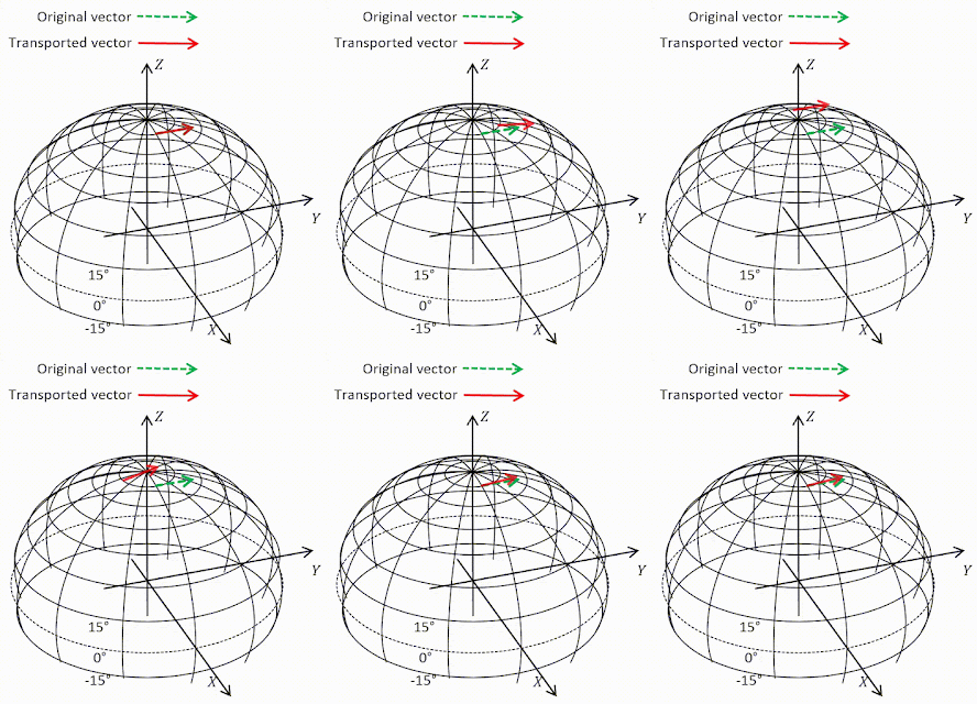
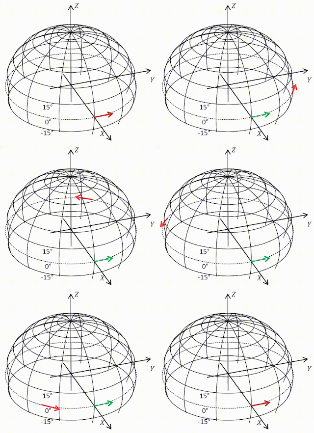
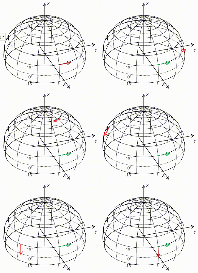
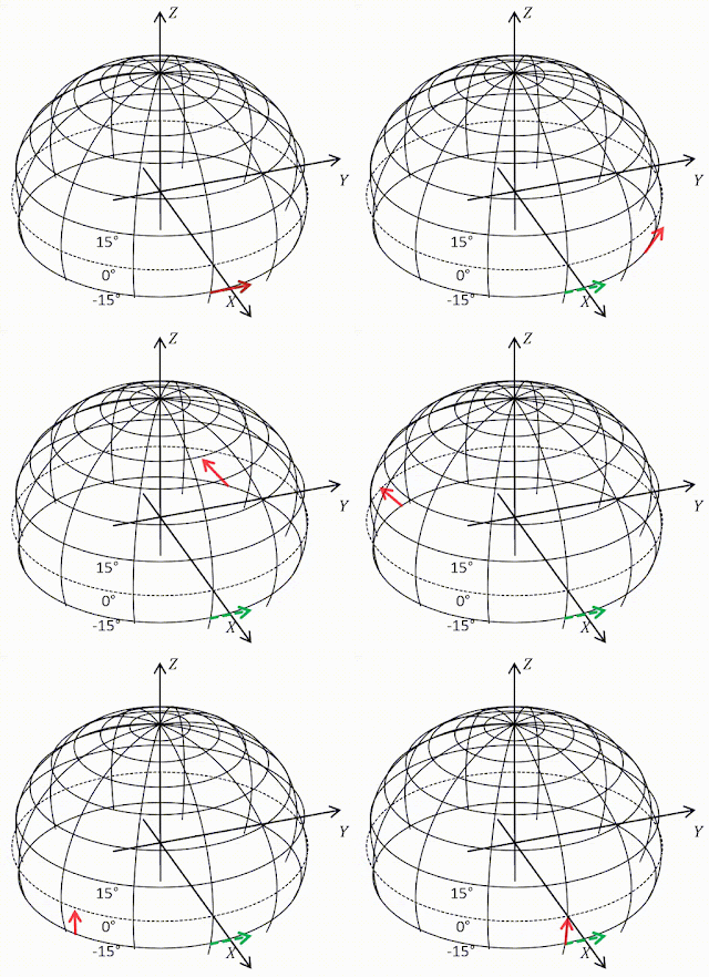
Vectors transported round latitudes calculated by parallel propagator

Note vector length never changes. ##T_n## was evaluated to 5 decimal places. 
Transport at 80°N. Vector barely
changes because it's nearly flat up there.
##T_n=0## at ##n=25##

Transport round equator. Vector remains
parallel because equator is geodesic.
##T_n=0## at ##n=1##

Transport at 15°N.
Vector rotates down by 87°.
##T_n=0## at ##n=11##


Transport at 15°S.
Vector rotates up by 87°.
##T_n=0## at ##n=11##


Thursday, 9 September 2021

MTW Ex 8.1 Practice with tensor algebra

Question

Let ##t,x,y,z## be Lorentz coordinates in flat spacetime, and let $$r=\left(x^2+y^2+z^2\right)^\frac{1}{2}\ ,\ \theta=\arccos{\left(\frac{z}{r}\right)}\ ,\ \phi=\arctan{\left(\frac{y}{x}\right)}$$be the corresponding spherical coordinates. Then$$e_0=\frac{\partial\mathcal{P}}{\partial t}\ ,\ e_r=\frac{\partial\mathcal{P}}{\partial r}\ ,\ e_\theta=\frac{\partial\mathcal{P}}{\partial\theta}\ ,\ e_\phi=\frac{\partial\mathcal{P}}{\partial\phi}$$is a coordinate basis, and $$e_{\hat{0}}=\frac{\partial\mathcal{P}}{\partial t}\ ,\ e_{\hat{r}}=\frac{\partial\mathcal{P}}{\partial r}\ ,\ e_{\hat{\theta}}=\frac{1}{r}\frac{\partial\mathcal{P}}{\partial\theta}\ ,\ e_{\hat{\phi}}=\frac{1}{r\sin{\theta}}\frac{\partial\mathcal{P}}{\partial\phi}$$is a non-coordinate basis.
(a) Draw a picture of ##e_\theta,e_\phi,e_{\hat{\theta}},e_{\hat{\phi}}## at several different points on a sphere of constant ##t,r##.
(b) What are the one-form bases dual to these tangent-vector bases?
(c) What is the transformation matrix linking the original Lorentz frame to the spherical coordinate frame ##\left\{e_a\right\}##?
(d) Use this transformation matrix to calculate the metric components ##g_{\alpha\beta}## in the spherical coordinate basis and invert the result to get ##g^{\alpha\beta}##.
(e) Show that the non-coordinate basis ##\left\{e_{\hat{a}}\right\}## is orthonormal everywhere; i.e. that ##g_{\hat{\alpha}\hat{\beta}}=\eta_{\alpha\beta}##; i.e. that $$g=-\omega^{\hat{0}}\otimes\omega^{\hat{0}}+\omega^{\hat{r}}\otimes\omega^{\hat{r}}+\omega^{\hat{\theta}}\otimes\omega^{\hat{\theta}}+\omega^{\hat{\phi}}\otimes\omega^{\hat{\phi}}$$(f) Write the gradient of a function ##f## in terms of the spherical coordinate and noncoordinate bases.
(g) What are the components of the Levi-Civita tensor in the spherical coordinate and noncoordinate bases?

Answers

This exercise seems mainly to be concerned with putting the rules in Box 8.4 into practice. We meet a noncoordinate (anholonomic) basis. One of the features of these is that coordinates cannot be used to describe positions but you can use components to describe other tensors. So$$p^{\hat{\mu}}=\left(a,b,c,d\right)\equiv ae^{\hat{0}}+be^{\hat{r}}+ce^{\hat{\theta}}+de^{\hat{\phi}}$$is at best meaningless but$$g_{\hat{\alpha}\hat{\beta}}=\left(\begin{matrix}a&0&0&0\\0&b&0&0\\0&0&c&0\\0&0&0&d\\\end{matrix}\right)$$is valid and is the answer to (d) when ##a=-1,b=c=d=1## .

I found an excellent new way of  creating animated gifs. Which I used for the answer to (a) below. The diagrams for ##e_{\hat{\theta}},e_{\hat{\phi}}## are a good indication of (e).

Coordinate bases going round equator

Coordinate bases going over pole

Non-coordinate bases going round equator

Friday, 30 July 2021

Pythagoras's and Newton's formulas for 𝝅

This fun video by Veritasium gives the story of Pythagoras and Newton and ##\pi## but it doesn't go into details. I wanted to know more.

Pythagoras calculated ##\pi## by placing regular n-agons just inside and outside a unit circle and calculating their perimeters. Some examples are shown below.
Apparently he stopped at a 96-agon. I reckon the result he got was$$48\sqrt{2-2\sqrt{\frac{1}{2}+\frac{1}{2}\sqrt{\frac{1}{2}+\frac{1}{4}\sqrt{2+\sqrt3}}}}<\pi<\frac{96\sqrt{2-2\sqrt{\frac{1}{2}+\frac{1}{2}\sqrt{\frac{1}{2}+\frac{1}{4}\sqrt{2+\sqrt3}}}}}{\sqrt{2+2\sqrt{\frac{1}{2}+\frac{1}{2}\sqrt{\frac{1}{2}+\frac{1}{4}\sqrt{2+\sqrt3}}}}}$$It was accurate to four significant digits and not surprisingly he stopped! He didn't even have decimal numbers.

The second last person to use this method in anger was Ludolph van Ceulen in about 1600 who did a ##2^{62}##-agon and still only got 35 decimal places. Apparently it took him 25 years. Nutter.

Then along came Newton (about 1700) and he used calculus (which he had just invented) and the binomial theorem to get$$\pi\approx-\frac{3\sqrt3}{2}+6-\left(\frac{1}{4}+\frac{3}{320}+\frac{45}{53,760}+\frac{1,575}{22,855,680}\right)$$That's accurate to five significant digits and a good deal easier to calculate. The further you go the better it gets:
Here's how they did it Newtons formula for pi.pdf (10 pages).

Friday, 2 July 2021

2.5 Differential forms

Vector ##U## (solid) and
1-form ##\widetilde{U}## (dashed)
In section 2.5 of Misner, Thorne, Wheeler 'differential forms' or '1-forms' are introduced and there is soon a fairly elaborate recipe for constructing 1-forms ##\widetilde{U}## from a vector ##U##. I reproduce it below. I tried out the recipe on some of the sample vectors shown and it seemed to work. A one form ##\widetilde{U}## is shown as a set of planes, whose spacing is defined, and which have a positive sense, or direction, as shown by a dashed arrow (which is not a vector). It would seem that you could equally well show the 1-form by a dashed arrow perpendicular (in the Euclidean sense) to the planes whose direction and length would show the positive sense and the spacing of the planes of ##\widetilde{U}##. You can. And I implemented it in a spreadsheet and made the amusing gif on the right. Then I saw the joke.

The recipe

Figure 2.7. Several vectors, ##A,B,C,D,E##, and corresponding 1-forms ##\widetilde{A},\widetilde{B},\widetilde{C},\widetilde{D},\widetilde{E}##. The process of drawing ##\widetilde{U}## corresponding to a given vector ##U## is quite simple. 1) Orient the surfaces of ##\widetilde{U}## orthogonal to the vector ##U## . (Why? Because any vector ##V## that is perpendicular to ##U## must pierce no surfaces of ##\widetilde{U}## (##0=U\bullet V=U,V##) and must therefore lie in a surface of ##\widetilde{U}##.) 2) Space the surfaces of  ##\widetilde{U}## so the number of surfaces pierced by some arbitrary vector ##Y## (e.g., ##Y=U##) is equal to ##Y\bullet U##.

Note that in the figure the surfaces of ##\widetilde{B}## are, indeed, orthogonal to ##B##; those of ##\widetilde{C}## are, indeed, orthogonal to ##C##, etc. If they do not look so, that is because the reader is attributing Euclidean geometry, not Lorentz geometry, to the spacetime diagram. He should recall, for example, that because ##C## is a null vector, it is orthogonal to itself (##C\bullet C=0##), so it must itself lie in a surface of the 1-form  ##\widetilde{C}##. Confused readers may review spacetime diagrams in a more elementary text, e.g., Taylor and Wheeler (1966)."

Read it here, including punchline: 2.5 Differential forms.pdf. (6 pages)

Saturday, 26 June 2021

Wave packets


I have started to read Misner, Thorne and Wheeler's great tome on gravitation. It starts quite differently from Carroll by emphasizing a coordinate free view. (Pythagoras and Euclid proved a lot without coordinates which were popularized RenΓ© Descartes about 2000 years after them.) In section 2.5 MTW claim that the pattern of surfaces (named ##\widetilde{{k}}##) generated by a matter wave (aka De Broglie wave) provide the simplest example of 1-forms which we know are covariant vectors or vectors with indices downstairs. I need to revise my quantum mechanics and find a book on the internet by JD Cresser. I think it is a bit hand-wavey but it helps me understand a bit more. The first step is generating a wave packet from a regular sine wave (or similar). The wave packet will be a particle.

Cresser starts with a cosine wave with a wave number 5 so the equation is ##\psi=\cos{5x}##. In this case the wave number is the number of waves that fit in a length ##2\pi##. Sometimes it is then number per unit length. He then takes another wave with wave number 5.5. The '2 sine waves' image shows them both. You can see a patter emerging. That becomes clearer if you add them and divide by 2 as shown in '2 waves added'. It is the famous beat that is heard if two nearby notes are played at the same time. He then adds more, all with wave numbers in the range 4.75 to 5.25 and claims that by adding even more you will get a wave packet. That is not true! If you add in more and more waves the picture remains the same, there are always small bulges and the large bulges just move off into the remote distance. The range shown is for ##x=\pm65##. On the 9 wave picture there are large bulges at about ##x=\pm100,\pm200\ldots## and on the 17 wave picture at about ##x=\pm200,\pm400\ldots## (I checked three of those). Then something in his text suggested that I should add waves in a larger range and that does produce a wonderful wave packet.

With 999 waves and ##k## in the range 4 to 6 the picture improves and with a slightly larger range, 0 to 10, it is a pretty decent wave packet (although I think there might be another spike well off the chart - try it yourself!).

Numbers and wave generator at Wave packets.pdf (4 pages) 

Tuesday, 3 November 2020

Solar orbit plotter

Here's how the plotter works
Newton's second law is$$
\vec{F}=m\vec{a}
$$Newton's law of gravity is$$
\vec{F}=\frac{GMm}{r^2}
$$They give you two differential equations of motion in polar coordinates$$
\frac{d^2r}{dt^2}-r\left(\frac{d\theta}{dt}\right)^2=-\frac{GM}{r^2}
$$$$
2\frac{dr}{dt}\frac{d\theta}{dt}+r\frac{d^2\theta}{dt^2}=0
$$Kepler's laws are
  1. The orbit of a planet is an ellipse with the Sun at one of the two foci.
  2. A line segment joining a planet and the Sun sweeps out equal areas during equal intervals of time.
  3. The square of a planet's orbital period is proportional to the cube of the length of the semi-major axis of its orbit.
The second differential equation quickly gives you Kepler's second law. It is more difficult to get$$
r=\frac{P}{1+e\cos{\left(\theta-\phi\right)}}
$$That is a circle when ##e=0##, an ellipse when ##\left|e\right|<1##, a parabola when ##\left|e\right|=1## and a hyperbola when ##\left|e\right|>1##. ##\phi## is the angle of the axis of symmetry of the curve. ##P## is a magic constant. The equation gives you Kepler's first law. 

Newton must have been very pleased when he did those. Part of the job was inventing calculus! 

The initial conditions determine ##P,e,\phi##. That requires more work if you only know the initial position and velocity.

Full details (except inventing calculus) in Commentary 5.4 Orbital toypdf. (9 pages)
The spreadsheets for plotting the curves are at 
Commentary 5.4 Orbital toy.xlsm (with animation macros)

Wednesday, 19 August 2020

Einstein-Rosen bridges: Wormholes in Schwarzschild spacetime


Nearing the end of section 5.7 Carroll discusses wormholes connecting regions IV and I of the Kruskal diagram. These wormholes are also called  Einstein-Rosen bridges.

It was supposed to be impossible to travel between regions I and IV of the Kruskal diagram and here Carroll shows us how it can almost be done. He is very brief, his diagram is wrong, but luckily I found a paper by Peter Collas and David Klein which goes into much more detail and helped me understand. I was even able to plot diagrams of the wormhole which takes you from the depths of region IV to the depths of region I. Sadly there is never enough time and my plot is, admittedly, a bodge. The real calculations would be too complicated.

There is another way for an intrepid explorer from region I (where we live) to get a glimpse of region IV. After they cross the event horizon (the dashed line ##r=R_s##) they could look 'down and to the left' and they could see light coming in from region IV. They could even meet another explorer from region IV. However they could never tell us back in region I what they learnt and would eventually perish in the singularity.

Read it here Commentary 5.7a Wormholes.pdf (3 pages).

Saturday, 8 August 2020

Conformal Diagrams


Continuing my studies of conformal transformations and diagrams I move on to appendix H, follow Carroll's logic carefully and attempt to plot his conformal diagram of Minkowski space which he shows in Fig H.4 and I have copied above in the centre. My effort is on the right. The diagrams are similar except that the curves of constant ##t##, the Minkowski coordinate, have gradient 0 nowhere on his diagram and twice on mine. And for lines of constant ##r## the score is 1,3 (gradient ##\infty##). I was distressed. Carroll does not give explicit equations for the curves so there is quite a long chain of calculation to get them plotted. I triple checked it and could find no error so I ransacked the internet and found the short paper from from 2008 by Claude Semay, title "Penrose-Carter diagram for an uniformly accelerated observer". The first part is only about an inertial observer and Semay draws a conformal diagram for her with lines of constant ##t,r## just like mine. I have reproduced half his diagram on the left. So I think Carroll has made a mistake in his Figure H.4 - perhaps he just guessed at the curves!

Carroll lists the important parts of the diagram
##i^+=## future timelike infinity (##T=\pi,R=0##)
##i^0=## spatial infinity (##T=0,R=\pi##)
##i^-=## past timelike infinity (##T=-\pi,R=0##)
##J^+=## future null infinity (##T=\pi-R,0<R<\pi##)
##J^-=## past null infinity (##T=-\pi+R,0<R<\pi##)
Carroll use a symbol like ##\mathcal {J}## not ##J## which he calls "scri". It is hard to reproduce.

Conformal diagrams are spacetime diagrams with coordinates such that the whole of spacetime fits on a piece of paper and moreover light cones are at 45° everywhere. The latter makes it easy to visualize causality. Since Minkowski spacetime has 45° light cones, if coordinates can be found which have a metric which is a conformal transformation of the Minkowski metric, the job is done. The first part of appendix H is devoted to finding conformal coordinates for flat Minkowski spacetime, expressed in polar coordinates - presumably to ease our work later in spherically symmetrical manifolds such as Schwarzschild. So we start from that metric:$$
{ds}^2=-{dt}^2+{dr}^2+r^2\left({d\theta}^2+\sin^2{\theta}{d\phi}^2\right)
$$
On the way to finding conformal coordinates we tried coordinates$$
\bar{t}=\arctan{t}\ \ ,\ \ \bar{r}=\arctan{r}
$$which certainly pack spacetime into the range$$
-\frac{\pi}{2}<\bar{t}<\frac{\pi}{2}\ ,\ 0\le\bar{r}<\frac{\pi}{2}
$$as you will see below if you press the button. Carroll says it might be fun to draw the light cones on that, so I made a movie:
Light cone at various ##\bar{r}##

Carroll's Figure H.2 is also quite confusing. It does not show the ##u,v## axes and I naturally assumed that the ##u## axis pointed down and to the right. It does not. It does the opposite.

Read all the details at Commentary App H Conformal Diagrams.pdf (12 pages) 

Thursday, 16 April 2020

Eddington and Finkelstein take us into a black hole


In the first part of section 5.2 (two posts ago) it seemed to be impossible to get inside the Schwarzschild radius. In the second part we look at other coordinate systems and find the Eddington-Finkelstein coordinates which show us how. The metric then takes a different form (which says something about Birkhoff's theorem) and it does not have an infinity at the Schwarzschild radius (##r=2GM##). 

The properties of the function ##1-2GM/r## (which causes the trouble) frequently amaze. It keeps eating itself up which is very satisfactory.

Eddington-Finkelstein coordinates eliminate the time coordinate ##t## and introduce
$$v=t+r+2GM\ln{\left(\frac{r}{2GM}-1\right)}$$
so the relationship between ##v## and ##t## is complicated.

The image shows a light cone at various distances out from the centre at ##r=0## . The ingoing light beam always heads for the centre the outgoing beam can get away when ##r>2GM## but flips towards the centre once it originates at a distance less than the Schwarzschild radius (aka the event horizon). The closer the starting point is to the centre, the less room there is for manoeuvre. 

I am slightly dubious about the direction of the ingoing side of a light cone inside the Schwarzschild radius.

See why and check my maths: Commentary 5.6#2 Schwarzschild Black Holes.pdf (6 pages)

Monday, 23 March 2020

Precession of perihelion of Mercury

In 5.5, we continue our adventures from the previous section 5.4 where we calculated a few things from the Killing vectors and geodesics of the Schwarzschild metric. I learnt a good lesson about Killing vectors then that went over my head previously.

There are several amazing things in this section one group being mathematical dexterity and the other being the feats of astronomers. The latter have measured the precession of the perihelion of Mercury at ##{44}^{\prime\prime}  \text{per century}##. ##{44}^{\prime\prime}## is 44 seconds of an arc or 44 times 1/3600 degrees. That's about the angle that a soccer ball would subtend if it was one kilometer away and if you could see it. How did they do that?

Apparently we are following d'Inverno 1992, not Einstein, and we start with a differential equation for the orbit in terms of radial distance ##r## and affine parameter ##\lambda## and turn it into a simpler differential equation in terms of ##x\propto1/r## and azimuth ##\phi##. A crafty differentiation then makes the equation further collapse into the equation of an ellipse with a small perturbation, as witnessed by astronomers. Using more trigonometrical tricks we then solve the GR perturbation part and find a term in that which must correspond to the precession. A further trig trick gets us to "the equation for an ellipse with an angular period that is not quite ##2\pi##" and from that we extract the precession of the perihelion of Mercury. How did anybody think up all that?

The image shows the path of a Mercury that precesses about a million times faster than our own Mercury. I plotted it to check the  "the equation for an ellipse with an angular period that is not quite ##2\pi##". It is surprisingly accurate for such a large precession.

Read my attempts to follow Carroll at
Commentary 5.5 Precession of perihelia.pdf (7 pages)
Commentary 5.4 Geodesics of Schwarzschild.pdf (8 pages)


Sunday, 23 February 2020

Monday, 3 February 2020

Taylor and Maclaurin series

In section 1.10 Carroll Taylor-expands a Lagrangian. So I had a look at Taylor series. There is a very good article on Wikipedia about them.


In particular I looked at the Taylor series of 1/(1-x), polynomials especially 3rd order, sines and 'other functions' which states that they often converge to their Taylor series expansion which is a technique often used in physics.


I was able to proved that a 3rd order polynomial is its Taylor series, that is:$$
k_0+k_1x+k_2x^2+k_3x^3=\sum_{i=0}^{i=3}\left(\left(\sum_{n=i}^{n=3}{\frac{n!}{\left(n-i\right)!}k_na^{n-i}}\right)\left(\sum_{j=0}^{j=i}\frac{x^{i-j}\left(-a\right)^j}{j!\left(i-j\right)!}\right)\right)
$$The bit on the right is the Taylor series (after a bit of work) and there are many terms like  ##a^ix^j## which amazingly cancel each other out. I was not able to prove that any polynomial is its Taylor series as Wikipedia states.

The Taylor series for the sine function is $$
x-\frac{x^3}{3!}+\frac{x^5}{5!}-\frac{x^7}{7!}+\ldots
$$which is Madhava's sine series, the well known formula for ##\sin{x}##. It was discovered in the west by Isaac Newton (1670) and Wilhelm Leibniz (1676). Taylor prospered in the 1700's so perhaps he found it independently. But since Newton and Leibniz independently invented calculus and argued about who was first, they probably new quite a bit about Taylor and McLaurin series. However they were all preceded by Madhava of Sangamagrama (c. 1350 – c. 1425), the founder of the Kerala school of astronomy and mathematics, who proved it as recorded in 1530 in the Indian text the Yuktibhāṣā. The picture shows the sine Taylor series for terms up to ##{x^15}/{15!}##. Amazingly accurate!
Read it all in Commentary 1.10 Taylor and Maclaurin series.pdf (4 pages)

Thursday, 30 January 2020

Exercise SI.01 Simple Lagrangians

Line according to formula For values
##-25\leq t\leq 25, a,b,c,d##. 
Question
Derive Newton's first law in two dimensions using Hamilton's principle and the Euler-Lagrange equation. First do it in Euclidean ##x,y## coordinates then in polar ##r,\theta## coordinates.

Do it by filling in the gaps in the Wikipedia article on the subject as quoted below.

1) Prove that ##m\ddot{x}=0## follows from the Euclidean Lagrangian as at (1), (2)
2) Prove that the two Euler–Lagrange at (4),(5) produce the two equations given.
3) Prove that the solutions to those two equations are indeed (6) and (7)
4) Plot (6), (7) for values of ##a,b,c,d## showing that it is a straight line and that ##a## is the velocity, ##c## is the distance of the closest approach to the origin, and ##d## is the angle of motion. What is ##b##?
Extracts from the article:
In two Euclidean dimensions in the absence of a potential, the Lagrangian is simply equal to the kinetic energy
\begin{align}
L=\frac{1}{2}mv^2=\frac{1}{2}m\left({\dot{x}}^2+{\dot{y}}^2\right)&\phantom {10000}(1)\nonumber
\end{align}in orthonormal ##(x,y)## coordinates, where the dot represents differentiation with respect to the curve parameter (usually the time, ##t##). Therefore, upon application of the Euler–Lagrange equations, [to the ##x## coordinate]
\begin{align}
\frac{d}{dt}\left(\frac{\partial L}{\partial\dot{x}}\right)-\frac{\partial L}{\partial x}=0\ \ \Rightarrow\ \ m\ddot{x}=0&\phantom {10000}(2)\nonumber
\end{align}[The Lagrangian and the solution are the same for the ##y## coordinate.]

In polar coordinates ##(r,\theta)## the kinetic energy and hence the Lagrangian becomes
\begin{align}
L=\frac{1}{2}m\left({\dot{r}}^2+r^2{\dot{\theta}}^2\right)&\phantom {10000}(3)\nonumber
\end{align}[where ##x=r\cos{\theta}\ \ ,\ y=r\sin{\theta}##.]
The radial ##r## and ##\theta## components of the Euler–Lagrange equations become, respectively
\begin{align}
\frac{d}{dt}\left(\frac{\partial L}{\partial\dot{r}}\right)-\frac{\partial L}{\partial r}=0\ \Rightarrow\ \ \ddot{r}-r{\dot{\theta}}^2=0&\phantom {10000}(4)\nonumber\\
\frac{d}{dt}\left(\frac{\partial L}{\partial\dot{\theta}}\right)-\frac{\partial L}{\partial\theta}=0\ \Rightarrow\ddot{\theta}+\frac{2\dot{r}\dot{\theta}}{r}=0&\phantom {10000}(5)\nonumber
\end{align}The solution to those two equations is given by
\begin{align}
r=\sqrt{\left(at+b\right)^2+c^2}&\phantom {10000}(6)\nonumber\\
\theta=\tan^{-1}{\left(\frac{at+b}{c}\right)}+d&\phantom {10000}(7)\nonumber
\end{align}for a set of constants ##a,\ b,\ c,\ d##  determined by initial conditions. Thus, indeed, the solution is a straight line given in polar coordinates: ##a## is the velocity, ##c## is the distance of the closest approach to the origin, and ##d## is the angle of motion." It does not reveal what ##b## is.
Answer 
I struggled with this and question 2 for over a day until I worked out what was really happening and came to the very important observation in the pdf. This enabled me to move on in section 1.10.

To begin with I got this: The first term in (2) is
\begin{align}
\frac{d}{dt}\left(\frac{\partial L}{\partial\dot{x}}\right)=\frac{1}{2}m\frac{d}{dt}\left(\frac{\partial{\dot{x}}^2}{\partial\dot{x}}\right)=m\frac{d\dot{x}}{dt}=m\ddot{x}&\phantom {10000}(8)\nonumber
\end{align}and the second term is
\begin{align}
\frac{\partial L}{\partial x}=\frac{1}{2}m\frac{\partial}{\partial x}\left({\dot{x}}^2\right)=m\dot{x}\frac{\partial}{\partial x}\left(\dot{x}\right)=m\frac{dx}{dt}\frac{\partial}{\partial x}\left(\frac{dx}{dt}\right)=m\frac{d}{dt}\left(\frac{dx}{dt}\right)=m\ddot{x}&\phantom {10000}(9)\nonumber
\end{align}put those back into (2) and we get
\begin{align}
m\ddot{x}-m\ddot{x}=0&\phantom {10000}(10)\nonumber
\end{align}Which does not prove that ##m\ddot{x}=0##!!

To see all what went wrong and the vital observation, look in Ex SI.01 Simple Lagrangians.pdf (5 pages)

Friday, 24 January 2020

The energy-momentum tensor in SR

Fluid flow by Thierry Dugnolle
Many moons ago I had skipped the end of section 9 and all of section 10 in chapter 1. It is time to return to them and flat space time starting with the end of section 9 it looks at the energy-momentum tensor for a perfect fluid. I had written at the top of the page "? don't follow much of this from 1.116". Now I do. It shows how to get from that tensor to two well known classical (non-relativistic) equations in the non-relativistic limit: a continuity equation and the Euler equation from fluid dynamics. This gives us faith that the tensor is correct - even though I had not heard of either of these equations.

Along the way we find some tricks with four-velocity ##U^\mu={dx^\mu} / {d\tau}##, meet the projection tensor ##P_{\ \ \ \ \nu}^\sigma## which projects a vector orthogonal to another do some dimensional analysis and find out what energy density really is (I missed this in the book, or Carroll forgot to mention it). I had to consult the great Physics Forums on that and got liked for a facetious comment about measuring it in £sd πŸ˜€- I'm sure that oil companies must do it: kerosene is more valuable per kg than bunker fuel.

All the details here Commentary 1.9 Energy Momentum Tensor.pdf (6 pages)

Friday, 17 January 2020

Physics in curved spacetime

I've now started chapter 4 on Gravitation just in time for 2020. Very exciting!
Fools straight line
Carroll first states two formulas of Newtonian Gravity his 4.1 and 4.2$$
\mathbf{a}=-\nabla\Phi
$$where ##\mathbf{a}## is the acceleration of a body in a gravitational potential ##\Phi##. And Poisson's differential equation for the potential in terms of the matter density ##\rho## and Newton's gravitational constant ##G##:$$
\nabla^2\Phi=4\pi G\rho
$$I had a long pause thinking about the various formulas for the Laplacian ##\nabla^2## here.
How to these tie up with the old-fashioned laws? Newton's law of gravity is normally stated as$$
F=G\frac{m_1m_2}{r^2}
$$which combined with Newton's second law ##F=m\mathbf{a}## gives us the acceleration of a mass in the presence of another as$$
\mathbf{a}=G\frac{M}{r^2}
$$In exercise 3.6 we were given 'the familiar Newtonian gravitational potential'$$
\Phi=-\frac{GM}{r}
$$A bit of rough reasoning shows these are equivalent.

At his 4.4 Carroll states that the next equation gives the path of a particle subject to no forces$$
\frac{d^2x^i}{d\lambda^2}=0
$$If we solve it in polar coordinates for ##r,\theta## instead of ##x,y## Carroll says we get a circle and he cheekily suggests that we might think free moving particles follow that path. But the solution is $$
r=m\theta+k
$$where ##m,k## are constants. We can plot that and, obviously if ##m=0## we get a circle of radius ##k## but if ##m\neq0## we get other more interesting lines which are equally wrong. See above. Another error by Carroll, but only minor 😏. The next one is a corker.

Then we examine the equations in a near Newtonian environment and equation 4.13 ##g^{\mu\nu}=\eta^{\mu\nu}-h^{\mu\nu}## is wrong. The actual equation is obviously$$
g^{\mu\nu}=\eta^{\mu\nu}+h^{\mu\nu}
$$Properly 4.13 might be
$$
g^{\mu\nu}=\eta^{\mu\nu}-h_{\rho\sigma}\eta^{\mu\sigma}\eta^{\nu\rho}
$$which is true to first order and gives ##h^{00}=-h_{00}## which is used in the next section. If  one accepts the approximation that ##\eta## can be used to raise and lower indices on any object of order ##h## then that also gives us$$
g^{\mu\nu}=\eta^{\mu\nu}-h^{\mu\nu}
$$which says ##h^{\mu\nu}=0##. Oops! But it turns out it turns out that the sign on ##h^{\mu\nu}## is immaterial in this section. There is a full analysis in the pdf.

We soon arrive at the conclusion that in the near Newtonian environment we have the time, time component of the metric is $$
g_{00}=-1-2\Phi
$$which is also what we were given in Exercise 3.6.

Tuesday, 24 December 2019

Review chapter 3

Before we start I have again found a very important paragraph, it is the last in section 3.2 and describes how we have got from the beginning to here. The beginning was the concept of a set which became a manifold and we ended up with metrics and covariant derivatives!

After nearly getting to the end of chapter 3 I realised that my ideas about covariant derivatives needed refinement and that I did not really understand parallel transport. With the former it would seem that metric compatibility, ##\nabla_\mu g_{\lambda\nu}=0##, arises out of the Leibnitz rule and the demand that the covariant derivative is a tensor and is not an 'additional property' - with the caveat that the manifold in question has a metric with the usual properties. On the latter I was still hazy until I explored further in this review.

I still don't think I have mastered every detail of this chapter to section 8 on Killing vectors but one thing is clear: If you have a tensor field ##T\left(x^\mu\right)## which you can express in terms of coordinates ##x^\mu## and we consider two points ##x^\alpha,x^\beta## then if you parallel transport the tensor from ##x^\alpha## along a geodesic to ##x^\beta## and call it ##T\prime\left(x^\beta\right)## there, then in all likelihood ##T\prime\left(x^\beta\right)\neq T\left(x^\beta\right)## and in some sense at least ##T^\prime\left(x^\beta\right)=T\left(x^\alpha\right)##. I think. Equation (20) in the document is saying that for a vector.

The rest of chapter 3 was straightforward and finally we met the geodesic deviation equation $$
A^\mu=\frac{D^2}{dt^2}S^\mu=R_{\ \ \nu\sigma\rho}^\mu T^\nu T^\rho S^\sigma
$$##A^\mu## is the "relative acceleration of (neighbouring) geodesics", ##S^\mu## is a vector orthogonal to a geodesic (pointing towards its neighbour) and ##T^\mu## is a vector tangent to the geodesic. The equation expresses the idea that the acceleration between two neighbouring geodesics is proportional to the curvature and, physically, it is the manifestation of gravitational tidal forces.

The six page document repeats the above and reviews covariant derivatives, parallel transport and geodesics as shown in the video, Riemann and Killing. It's at Commentary 3 Review chapter 3.pdf.

Wednesday, 18 September 2019

Exercise 3.04 (with Spherical coordinates)

This is a model for doing the real exercise 3.4 which was on paraboloidal coordinates ##\left(u,v,\phi\right)##. I did it because I know, or can find, the answers and so I can check my methods. There is very little information on  paraboloidal coordinates that I can findπŸ˜–. I was particularly hazy on how to calculate the basis vectors. Now I know! It appears that basis one-forms point in the same direction as basis vectors and the ##r## basis one-form is the same as the vector. I probably should think about that harder. I also had quite a lot of problems with signs on terms such as ##\sqrt{x^2+y^2}##. Inattentive use of https://www.derivative-calculator.net/ gave wrong answers.

Hopefully I will very soon complete the nasty real question.


Question

In Euclidean three-space we can define spherical coordinates ##\left(r,\theta,\phi\right)## via
\begin{align}
x=r\sin{\theta}\cos{\phi}&\phantom {10000}(1)\nonumber\\
y=r\sin{\theta}\sin{\phi}&\phantom {10000}(2)\nonumber\\
z=r\cos{\theta}&\phantom {10000}(3)\nonumber
\end{align}Note: we are using the 'physicist' convention as shown on the video. ## \theta## is the colatitude (polar) and ## \phi## the longitude (azimuthal).

(a) Find the coordinate transformation matrix between paraboloidal and Cartesian coordinates ##\frac{\partial x^\alpha}{\partial x^{\beta^\prime}}## and the inverse transformation. Are there any singular points in the map?

(b) Find the basis vectors and the basis one-forms in terms of Cartesian basis vectors and forms.

(c) Find the metric and inverse metric in paraboloidal coordinates.

(d) Calculate the Christoffel symbols.

(e) Calculate the divergence ##\nabla_\mu V^\mu## and Laplacian ##\nabla_\mu\nabla^\mu f##.

Full details at Ex 3.04 Spherical coordinates.pdf. 7 pages including link to Excel file for generating the video.