Powers of sine and cosine as multiple angles

I had a problem which required integrating powers of sines and cosines. 

I used integral-calculator to do the work up to a power of six. Its results are shown below. $$\fbox{$\begin{matrix}n&\int{\cos^n{\theta}d\theta}&\int{\sin^n{\theta}d\theta}\\2&\frac{\sin{\left(2\theta\right)}+2\theta}{4}&\frac{-\sin{\left(2\theta\right)}+2\theta}{4}\\3&\sin{\theta}-\frac{\sin^3{\theta}}{3}&\frac{\cos^3{\theta}}{3}-\cos{\theta}\\4&\frac{\sin{\left(4\theta\right)}+8\sin{\left(2\theta\right)}+12\theta}{32}&\frac{\sin{\left(4\theta\right)}-8\sin{\left(2\theta\right)}+12\theta}{32}\\5&\frac{\sin^5{\theta}}{5}-\frac{2\sin^3{\theta}}{3}+\sin{\theta}&-\frac{\cos^5{\theta}}{5}+\frac{2\cos^3{\theta}}{3}-\cos{\theta}\\6&\frac{\sin{\left(6\theta\right)}+9\sin{\left(4\theta\right)}+45\sin{\left(2\theta\right)}+60\theta}{192}&-\frac{\sin{\left(6\theta\right)}-9\sin{\left(4\theta\right)}+45\sin{\left(2\theta\right)}-60\theta}{192}\\\end{matrix}$}$$

There appears to be a pattern. But at the moment it is veiled. The integrals of odd powers can be found by a crafty substitution which I found here. It gives$$\int\sin^n{\theta}d\theta=\sum_{l=0}^{l=\frac{n-1}{2}}{\left(-1\right)^{l+1}B_l^{\frac{n-1}{2}}}\frac{\cos^{2l+1}{\theta}}{2l+1}+C,\ for\ odd\ n$$$$\int\cos^n{\theta}d\theta=\sum_{l=0}^{l=\frac{n-1}{2}}{\left(-1\right)^lB_l^{\frac{n-1}{2}}\frac{\sin^{2l+1}{\theta}}{2l+1}}+C,\ for\ odd\ n$$where ##B_l^n## is the binomial coefficient$$B_l^n=\frac{n!}{l!\left(n-l\right)!}$$The integrals of even powers are not so simple. I ventured into multiple angle expressions for ##\cos^n{\theta},\sin^n{\theta}## using the Chebyshev method. Multiple angles are easy integrate. I ended up with the Christmas trees at the top.

If you're interested read it here: Sine and Cosine formulas.pdf (12 pages).

The Parallel Propagator and using it on the surface of a sphere

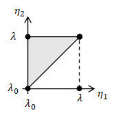
The three page Appendix I is on the parallel propagator which gives a general solution to the parallel transport equation of a vector. The appendix shows how to get this from the parallel transport equation which is, for a vector ##V^\nu## transported along a curve ##x^\mu\left(\lambda\right)## $$\frac{dx^\mu}{d\lambda}\partial_\mu V^\nu+\frac{dx^\mu}{d\lambda}\Gamma_{\mu\sigma}^\nu V^\sigma=0$$First we note that the transported vector can be calculated by$$V^\mu\left(\lambda\right)=P_{\ \ \rho}^\mu\left(\lambda,\lambda_0\right)V^\rho\left(\lambda_0\right)$$where ##V^\rho\left(\lambda_0\right)## is the vector at the start point ##x^\mu\left(\lambda_0\right)## and ##P_{\ \ \rho}^\mu\left(\lambda,\lambda_0\right)## is some matrix which is called the parallel propagator. Next we define another matrix $$A_{\ \ \rho}^\mu\left(\lambda\right)=-\Gamma_{\sigma\rho}^\mu\frac{dx^\sigma}{d\lambda}$$and then show that (dropping indices on the matrices)$$P\left(\lambda,\lambda_0\right)=I+\sum_{n=1}^{n=\infty}T_n$$where ##I## is the identity matrix and $$T_n=\int_{\lambda_0}^{\lambda}{\int_{\lambda_0}^{\eta_n}\int_{\lambda_0}^{\eta_{n-1}}{\ldots\int_{\lambda_0}^{\eta_2}A\left(\eta_n\right)A\left(\eta_{n-1}\right)\ldots A\left(\eta_1\right)}d^n\eta}$$$$=\frac{1}{n!}\int_{\lambda_0}^{\lambda}{\int_{\lambda_0}^{\lambda}\int_{\lambda_0}^{\lambda}{\ldots\int_{\lambda_0}^{\lambda}\mathcal{P}\left[A\left(\eta_n\right)A\left(\eta_{n-1}\right)\ldots A\left(\eta_1\right)\right]}d^n\eta}$$where ##\mathcal{P}## orders the matrices ##A\left(\eta_i\right)## so that ##\eta_n\geq\eta_{n-1}\geq\ldots\geq\eta_1##.

2-simplex

The first integral is over ##n##-dimensional equilateral right triangles, or ##n##-simplices and is quite hard to calculate but ##n!## ##n##-simplices make an ##n##-cube which makes the second integral which is much easier to calculate. I had a bit of trouble getting my head round all that and I tested it on a few examples including vectors transported along lines of constant latitude.  It all works!

Read about it here Commentary App I Parallel Propagator.pdf (13 pages). 

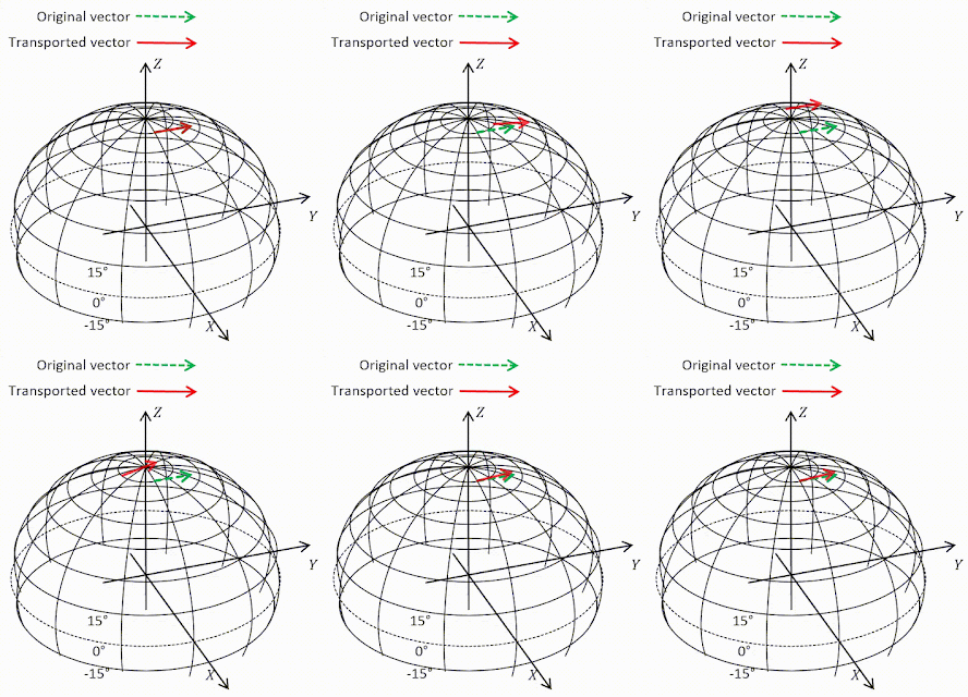
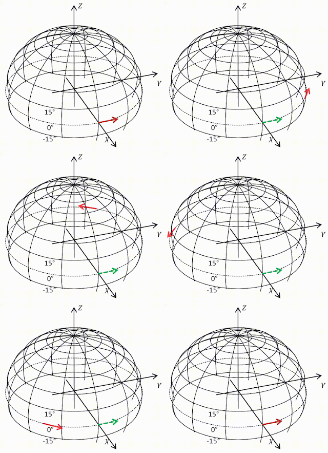
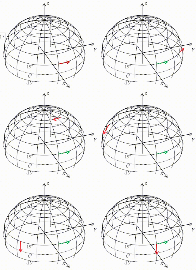
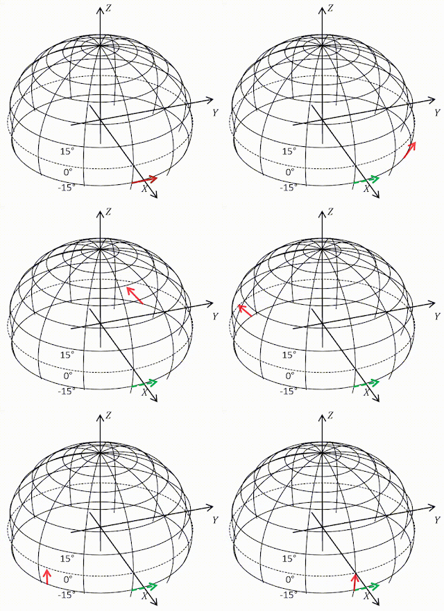
Vectors transported round latitudes calculated by parallel propagator

Note vector length never changes. ##T_n## was evaluated to 5 decimal places. 

Transport at 80°N. Vector barely
changes because it's nearly flat up there.
##T_n=0## at ##n=25##

Transport round equator. Vector remains
parallel because equator is geodesic.
##T_n=0## at ##n=1##

Transport at 15°N.
Vector rotates down by 87°.
##T_n=0## at ##n=11##

Transport at 15°S.
Vector rotates up by 87°.
##T_n=0## at ##n=11##

MTW Ex 6.2,3.1 Commutators and partial derivatives

Question

Take the mathematician's view that tangent vectors and directional derivatives are the same thing, ##u\equiv\partial_u##. Let ##u,v## be two vector fields and define their commutator in the manner familiar from quantum mechanics [not familiar to me!]$$\left[u,v\right]\equiv\left[\partial_u,\partial_v\right]\equiv\partial_u\partial_v-\partial_v\partial_u$$(a) Derive the following expression for ##\left[u,v\right]## valid in any coordinate basis$$\left[u,v\right]=\left(u^\beta v_{\ \ ,\beta}^\alpha-v^\beta u_{\ \ ,\beta}^\alpha\right)e_\alpha$$Thus despite that it looks like a second-order differential operator, ##\left[u,v\right]## is actually of first order - i.e. it is a tangent vector. 

(b) For any basis ##\left\{e_\alpha\right\}## one defines the "commutation coefficients" ##c_{\beta\gamma}^{\ \ \ \ \ \alpha}## and ##c_{\beta\gamma\alpha}## by $$\left[e_\beta,e_\gamma\right]\equiv c_{\beta\gamma}^{\ \ \ \ \ \alpha}e_\alpha;\ \ c_{\beta\gamma\alpha}=g_{\alpha\mu}c_{\beta\gamma}^{\ \ \ \ \ \mu}$$Show that ##c_{\beta\gamma}^{\ \ \ \ \ \alpha}=c_{\beta\gamma\alpha}=0## got any coordinate basis.

(c) Calculate ##c_{\hat{\beta}\hat{\gamma}}^{\ \ \ \ \ \hat{\alpha}}## for the spherical noncoordinate basis of exercise 8.1.

Answers

This was straight forward. But I learned that Hermann Schwarz outshone Euler,  Lagrange, Cauchy who were all very clever. It was Schwarz who proved that partial derivatives commute. The others didn't get it quite right apparently. So I repeated his proof and now I know when partial derivatives commute and when they don't. Hurrah.

On this exercise: 8.2 Exercise Commutators.pdf (3 pages)

On Schwarz's theorem: 8.2 Schwarz's theorem.pdf (4 pages)

And a bonus: 3.1 Exercise Components of EMF tensor.pdf (2 pages) 

Kinetic Energy ≠ ½mv²

While studying ##E=mc^2## I keep noticing that kinetic energy is not ##\frac{1}{2}mv^2## as we were always taught in school. The relativistic formula is, in various forms, $$K_{rel}=\frac{c^3}{\sqrt{c^2-v^2}}-c^2=c^2\left(\frac{1}{\sqrt{1-\beta^2}}-1\right)=c^2\left(\frac{1}{2}\beta^2+\frac{3}{8}\beta^4+\ldots\right)$$where ##\beta=v/c##.

On May 2nd 2021 the Parker Solar Probe achieved a velocity of 532,000 km/h which is about ##0.0005c##. That gives

\begin{align}\frac{K_{rel}}{c^2}=1.25000023\times{10}^{-7}\ ,\ \frac{K_{cl}}{c^2}=1.25\times{10}^{-7}&\phantom {10000}(8)\nonumber\end{align}Not much difference. The mass of the probe is about 600kg so the difference is ##2.3\times{10}^3\ Joules## which might keep a phone going for an hour.

 

The difference is more noticeable at much higher velocities. At ##0.1c## the difference is about 1%. It goes wild as you approach the speed of light.

A bit more here: 2.2 Kinetic energy.pdf (1 page)

Why does E=mc²?

Trying to follow the second worked example in Box 2.2 of Misner, Thorne, Wheeler I realised that I did not know how Einstein proved ##E=mc^2## and, when I checked in my books, both MWT and Carroll gloss it over! Using Einstein's 1905 paper, an internet video and the relativistic Doppler shift formulas given by Wikipedia I now do. Here's my version based on those.

We take two scenarios 

1) observe the object, in its rest frame, emitting two pulses of light with energy ##E/2## in opposite directions so that it does not change velocity and then we take off in a rocket with velocity ##v## so the object has some kinetic energy ##K_1## 

2) measure its kinetic energy ##K_2## from a frame moving with velocity ##v## then it emits the light which will have energy doppler shifted according to $$E_r=E\left(1+\frac{v^2}{2c^2}\right)$$After the emission we are now in the final state of scenario 1 and the object must have kinetic energy ##K_1## and total energy ##K_1-E##.

In both scenarios the object lost energy by radiation and gained kinetic energy (because the observer started moving) and we end up at the same place. The total energy must be the same in either scenario therefore$$K_1-E=K_2-E\left(1+\frac{v^2}{2c^2}\right)\Rightarrow\frac{Ev^2}{2c^2}=K_2-K_1$$We know how to calculate the kinetic energy (##mv^2/2##) and the velocities of the kinetic energies are the same so the masses must have changed. So$$\frac{Ev^2}{2c^2}=m_2\frac{v^2}{2}-m_1\frac{v^2}{2}\Rightarrow E=\Delta Mc^2$$where ##\Delta M## is the change in the mass of the object. Furthermore we conclude that if one could get all the energy out of an object of mass ##m## that energy would be

$$E=mc^2$$For more details including the derivation of ##E_r## see the very short 2.2 Box E=mc2.pdf.

Coming soon. More on that Box 2.2.

2.5 Differential forms

Vector ##U## (solid) and
1-form ##\widetilde{U}## (dashed)

In section 2.5 of Misner, Thorne, Wheeler 'differential forms' or '1-forms' are introduced and there is soon a fairly elaborate recipe for constructing 1-forms ##\widetilde{U}## from a vector ##U##. I reproduce it below. I tried out the recipe on some of the sample vectors shown and it seemed to work. A one form ##\widetilde{U}## is shown as a set of planes, whose spacing is defined, and which have a positive sense, or direction, as shown by a dashed arrow (which is not a vector). It would seem that you could equally well show the 1-form by a dashed arrow perpendicular (in the Euclidean sense) to the planes whose direction and length would show the positive sense and the spacing of the planes of ##\widetilde{U}##. You can. And I implemented it in a spreadsheet and made the amusing gif on the right. Then I saw the joke.

The recipe

Figure 2.7. Several vectors, ##A,B,C,D,E##, and corresponding 1-forms ##\widetilde{A},\widetilde{B},\widetilde{C},\widetilde{D},\widetilde{E}##. The process of drawing ##\widetilde{U}## corresponding to a given vector ##U## is quite simple. 1) Orient the surfaces of ##\widetilde{U}## orthogonal to the vector ##U## . (Why? Because any vector ##V## that is perpendicular to ##U## must pierce no surfaces of ##\widetilde{U}## (##0=U\bullet V=U,V##) and must therefore lie in a surface of ##\widetilde{U}##.) 2) Space the surfaces of  ##\widetilde{U}## so the number of surfaces pierced by some arbitrary vector ##Y## (e.g., ##Y=U##) is equal to ##Y\bullet U##.

Note that in the figure the surfaces of ##\widetilde{B}## are, indeed, orthogonal to ##B##; those of ##\widetilde{C}## are, indeed, orthogonal to ##C##, etc. If they do not look so, that is because the reader is attributing Euclidean geometry, not Lorentz geometry, to the spacetime diagram. He should recall, for example, that because ##C## is a null vector, it is orthogonal to itself (##C\bullet C=0##), so it must itself lie in a surface of the 1-form  ##\widetilde{C}##. Confused readers may review spacetime diagrams in a more elementary text, e.g., Taylor and Wheeler (1966)."

Read it here, including punchline: 2.5 Differential forms.pdf. (6 pages)

Wave packets

I have started to read Misner, Thorne and Wheeler's great tome on gravitation. It starts quite differently from Carroll by emphasizing a coordinate free view. (Pythagoras and Euclid proved a lot without coordinates which were popularized René Descartes about 2000 years after them.) In section 2.5 MTW claim that the pattern of surfaces (named ##\widetilde{{k}}##) generated by a matter wave (aka De Broglie wave) provide the simplest example of 1-forms which we know are covariant vectors or vectors with indices downstairs. I need to revise my quantum mechanics and find a book on the internet by JD Cresser. I think it is a bit hand-wavey but it helps me understand a bit more. The first step is generating a wave packet from a regular sine wave (or similar). The wave packet will be a particle.

Cresser starts with a cosine wave with a wave number 5 so the equation is ##\psi=\cos{5x}##. In this case the wave number is the number of waves that fit in a length ##2\pi##. Sometimes it is then number per unit length. He then takes another wave with wave number 5.5. The '2 sine waves' image shows them both. You can see a patter emerging. That becomes clearer if you add them and divide by 2 as shown in '2 waves added'. It is the famous beat that is heard if two nearby notes are played at the same time. He then adds more, all with wave numbers in the range 4.75 to 5.25 and claims that by adding even more you will get a wave packet. That is not true! If you add in more and more waves the picture remains the same, there are always small bulges and the large bulges just move off into the remote distance. The range shown is for ##x=\pm65##. On the 9 wave picture there are large bulges at about ##x=\pm100,\pm200\ldots## and on the 17 wave picture at about ##x=\pm200,\pm400\ldots## (I checked three of those). Then something in his text suggested that I should add waves in a larger range and that does produce a wonderful wave packet.

With 999 waves and ##k## in the range 4 to 6 the picture improves and with a slightly larger range, 0 to 10, it is a pretty decent wave packet (although I think there might be another spike well off the chart - try it yourself!).

Numbers and wave generator at Wave packets.pdf (4 pages) 

Cosmic distance measures

 I am still trying to prove the relationships between different cosmic distance measures$$d_L=\left(1+z\right)d_M=\left(1+z\right)^2d_A$$and I'm sill not there. on the way I came across a nice graph on Wikipedia comparing them for various ##z## and wondered if I could reproduce it. My version and the Wikipedia one are shown below, I was pleased.

Spot the difference

Here's how and my first attempts at proving that formula: Commentary 8.5.4 More distances.pdf (10 pages)

Three years old

The very first post on this blog was on Thursday, 15 March 2018. So we're over three years old and now getting nearly 3,000 pageviews per month. There was a mysterious big uptick in September last year. 

adpushup.com says that I might get $70 per year from adverts. google.com/adsense says 5,000€. Dreaming.

Thanks to all you readers!

Luminosity distance

In section 8.5 we are looking at redshifts and distances. We started in an FLRW universe with metric

\begin{align}{ds}^2=-{dt}^2+a^2\left(t\right)\left[\frac{{\rm dr}^2}{1-\kappa r^2}+r^2{d\theta}^2+r^2\sin^2{\theta}{d\phi}^2\right]&\phantom {10000}(1)\nonumber\end{align}or

\begin{align}{ds}^2=-{dt}^2+a^2\left(t\right){R_0}^2\left[{d\chi}^2+{S_k}^2\left(\chi\right){d\Omega}^2\right]&\phantom {10000}(2)\nonumber\end{align}where ##k\in\left\{-1,0,1\right\}## and

\begin{align}S_k\left(\chi\right)\ \equiv\left\{\begin{matrix}\sin{\chi},&k=+1&\rm{closed}\\\chi,&k=0&\rm{flat}\\\sinh{\chi}&k=-1&\rm{open}\\\end{matrix}\right.&\phantom {10000}(3)\nonumber\end{align}(2) is Carroll's 8.106, a sort of hybrid FLRW metric.

This starts at Carroll's 8.110 where he defines distance luminosity ##d_L## which you can get if you know the absolute luminosity of a star (or galaxy) and can measure the amount of light that reaches you. We then correct that for the expansion of the universe and further correct it because the universe deviates from a perfect sphere according to ##S_k\left(\chi\right)##. We arrive at the celebrated and complicated formula at (4) which uses (5) which uses (6) .

\begin{align}d_L=\left(1+z\right)\frac{{H_0}^{-1}}{\sqrt{\left|\Omega_{c0}\right|}}S_k\left[\sqrt{\left|\Omega_{c0}\right|}\int_{0}^{z}\frac{dz^\prime}{E\left(z^\prime\right)}\right]&\phantom {10000}(4)\nonumber\end{align}where

\begin{align}E\left(z\right)=\left[\sum_{i(c)}{\Omega_{i0}\left(1+z\right)^{n_i}}\right]^\frac{1}{2}&\phantom {10000}(5)\nonumber\end{align}and there are four elements in the summation, one each for matter, radiation, curvature and vacuum energy density. ##\Omega_i## is the density parameter which we met before and was defined as 

\begin{align}\Omega_i=\frac{8\pi G}{3H^2}\rho_i&\phantom {10000}(6)\nonumber\end{align}where the ##\rho_i## are the energy densities for each of those four things. ##\Omega_i## and ##H##, the Hubble factor acquire a 0 subscript for their values in the present epoch. 

I then try to calculate (4) from known values. ##\Omega_{c0}## the pseudo-density parameter for curvature comes from Friedmann's equation and the other three density parameters. That radiation energy is negligible, matter energy density corresponds to what is usually called ordinary (baryonic) plus dark matter and vacuum energy density is dark energy. The integral in (4) must be calculated numerically and I plotted below (page 10 in the pdf). After that we have plots of luminosity distance vs redshift for the three kinds of universe determined by ##k## in (3). Luminosity distances greater 100 billion light years are quite easy to get. I thought everything was a failure until I found some distance calculators which gave more or less the same! According to Carroll, these distances are compared with those measured from absolute and apparent luminosity. Luminosity distance is mighty peculiar. Coming soon: Proper motion distance and Angular diameter distance.

I also found that there is a missing divide by sign in Carroll's equation 8.122.

Read all about it at Commentary 8.5.2 Redshifts and Distances.pdf (12 pages)

Super Nova

Kepler's Supernova* remnant in background

There is a unified catalogue of 5526 supernova (SN) by D. Lennarz et al and I want to extract the Type Ia Super Novae along with their magnitudes, redshifts and distances to see how those compare with what I have been learning out about redshifts and luminosity and other distances in section 8.3. Type Ia Super Nova are all supposed to have the same absolute magnitude of −19.3 (about 5 billion times brighter than the Sun). I was able to confirm Hubble's law and learnt that that the mighty peculiar formula for Type Ia Supernova: ##m=5\log_{10}{D}-24.3## for the fall off in apparent magnitude ##m## with distance ##D## is in fact an inverse power law. And that corrections for the expansion and curvature of the universe at this range (about a fifteenth of the size of the visible universe) are immaterial. 

Read all about it at Commentary 8.5.3 Super Nova.pdf (4 pages)

* Kepler's supernova was the last one ever seen in the Milky Way. That was 1604. It would be exciting if there was another one soon. (But not too close!)

Redshifts and Distances

Still working on the magic Killing tensor ##K_{\mu\nu}=a^2\left(g_{\mu\nu}+U_\mu U_\nu\right)## in FLRW spacetime:

• We use ##K_{\mu\nu}## to show that interstellar gas cools in an expanding universe.
• Then we use it to show that as the universe expands the observed frequency of a photon will decrease. 
• Cosmologist measure the redshift, ##z##, of distant objects and we show how this tells us the scale factor ##a## when the object emitted the light being measured. 
• I then looked up some galactic distances and redshifts to compare them (pictured). Extrapolating the graph indicates the size of the visible universe is ~15 Gly.
• Carroll then seems to ramble a bit and goes back to a non-relativistic redshift. The history of Doppler and Hubble, which he does not mention, is quite interesting.
• Getting back on track Carrol shows that the nearby universe can be thought of as flat and we are able to use proper distance meaningfully and derive Hubble's law. I think he is overcomplicated.
• Next step other distances!

Read it here Commentary 8.5 Redshifts and Distances.pdf (9 pages)

A Killing Tensor in FLRW spacetime

God (or the universe) was playing tricks on me last week. In section 8.5 we are looking at redshifts and distances. The latter are more complicated than you might thing. 

I have got to the end of the first paragraph in this section and ignited a controversy on Physics Forums about ##a## the scale factor which tells you how much the universe is expanding. The question is: Is the scale factor a scalar?

We start in an FLRW universe with metric$$
{ds}^2=-{dt}^2+a^2\left(t\right)\left[\frac{{\rm dr}^2}{1-\kappa r^2}+r^2{d\theta}^2+r^2\sin^2{\theta}{d\phi}^2\right]
$$First Carroll invents a tensor$$
K_{\mu\nu}=a^2\left(g_{\mu\nu}+U_\mu U_\nu\right)
$$where ##U^\mu=\left(1,0,0,0\right)## is the 4-velocity of (all) comoving observers. Carroll says it satisfies $$
\nabla_{(\sigma}K_{\mu\nu)}=0
$$"as you can check" and therefore it is a Killing tensor. I accepted the challenge and it took me a few days.

I was not sure if the scale factor ##a## is a scalar. If it's not then it is doubtful whether ##K_{\mu\nu}## is even a tensor. If ##a## is not a scalar but somehow ##K_{\mu\nu}## is a tensor then we must calculate ##\nabla_\sigma K_{\mu\nu}## by expanding the covariant derivative:$$
\nabla_\sigma K_{\mu\nu}=\mathrm{\partial}_\sigma K_{\mu\nu}-\Gamma_{\sigma\mu}^\lambda K_{\lambda\nu}-\Gamma_{\sigma\nu}^\lambda K_{\mu\lambda}
$$If ##a## is a scalar then we can use the Leibniz rule: $$
\nabla_\sigma K_{\mu\nu}=\left(g_{\mu\nu}+U_\mu U_\nu\right)\nabla_\sigma\left(a^2\right)+a^2\nabla_\sigma\left(g_{\mu\nu}+U_\mu U_\nu\right)
$$I used Leibniz first and failed. Then I was inspired by a simpler version on physics.stackexchange and got the right answer using the first formula. That made me doubt that ##a## was a scalar. So I asked about it on Physics Forums. Then I found my error in the Leibniz method and it gave the right answer! So now I think that ##a## is a scalar after all. The Leibniz way is a good deal more efficient than the first.  The discussion continues and I think that PeterDonis has had the last word although vanhees71 is still wriggling at ##11. He surrenders at #13.

Read it all at Commentary 8.5 Killing Tensor in FLRW spacetime.pdf. (7 pages)

Cosmological vs Doppler redshift

Milne Universe. Flat and expanding.

I want to compare Carroll's section 3.5 where he "demonstrates the conceptual distinction between  the cosmological redshift and the conventional Doppler effect" and Orodruin's Physics Forums Insight were he concludes "I have seen many instances where people in popular texts make a very strong claim that cosmological redshift is fundamentally different from Doppler shift. The computations above clearly show that this is not the case, instead cosmological redshift and Doppler shift are two sides of the same coin, just viewed in different coordinates."

Let's see whether Carroll is one of the guilty ones writing popular texts or if his "conceptual distinction" is just a matter of reference frames.

My first attempt at this was in September 2019 and I got told by Orodruin to read his Insight on Physics Forums. I was (correctly) daunted and postponed the reading. My next attempt was in November 2019, while travelling, but time and place defeated me. At last after nearly 1½ years I have won.

I followed most of Orodruin's insight. His approximation for the mapping from Minkowski to FLRW coordinates was the most difficult part for me. I make some effort to check its validity. With that under his belt he briskly derives Hubble's law in Minkowski coordinates showing that there are (at least) two ways of looking at the expansion of the universe. The punch line comes at the end with his pathological example (a Milne universe, pictured) where he shows, without approximations, that the only distinction between cosmological and Doppler redshift is the frame of reference used. 

Carroll's thought experiment showing a "conceptual distinction" between them involved some very unreal events: Galaxies are started and stopped in a Minkowski frame and FLRW expansion is turned on and off. I have not pinned down exactly what is wrong with that but Orodruin's method is much more real. I am convinced.

On the way I learnt 

• more about Taylor series which I find peculiar.
• that coordinates are orthogonal if the metric is diagonal and I now almost understand the notation ##e_\tau=\partial_t##.
• about proper distance and simultaneity conventions, which I had never heard of before.
• I learnt about the varying speed of light!

I made notes about all these. It was an enlightening three weeks.

Read it all at Commentary 3.5 Expanding Universe Revisited #3.pdf.

Photon sphere

M87* By Event Horizon Telescope

I come across the photon sphere (or last photon orbit) which is another radius around a Schwarzschild black hole at a distance ##3R_s/2##. It is the closest distance for a stable orbit and light would orbit there in an exact circle. I would like to calculate it using Carroll conventions. ##R_s=2GM## is the Schwarzschild radius.

There is a Wikipedia article on it. The proof it gives has some peculiarities. I followed it avoiding those. It is one page.
Here: Commentary 5.4 Photon Sphere.pdf 

The famous picture is of M87* the black hole in our neighbour galaxy Messier 87. The black central sphere has a radius of ##2.6R_s## so the photon sphere is well inside that black bit and this is not a good illustration of a photon sphere!

Tensor Tricks

Cat gets Carroll

The file Commentary Tensor Tricks.pdf contains some useful equations for tensor manipulation which I have collected. 

The very first on tensor rank comes from early in the book (page 21) where we are told that: a tensor ##T## of type (or rank) ##\left(k,l\right)## is a multilinear map from a collection of dual vectors and vectors to ##\mathbf{R}##: 

$$T:\left(T_p^\ast\times\cdots\times T_p^\ast\right)_{k\ times}\times\left(T_p\times\cdots\times T_p\right)_{l\ times}\rightarrow\mathbf{R}$$

That is Carroll's 1.56 and I am pretty sure he has that the wrong way round. It should say: a tensor ##T## of type (or rank) ##\left(k,l\right)## is a multilinear map from a collection of ##k## vectors and ##l## dual vectors to  ##\mathbf{R}##:$$T:\left(T_p\times\cdots\times T_p\right)_{k\ times}\times\left(T_p^\ast\times\cdots\times T_p^\ast\right)_{l\ times}\rightarrow\mathbf{R}$$But it turns out that you don't really need to know what ##k## and ##l## are separately in General Relativity (because we always have a metric). You only need to know the total rank ##k+l##!

Contents

• What tensor rank?
• Multi-dimensional Chain Rule
• Partial derivative gives Kronecker delta: Coordinates, Vectors, Tensors
• Partial derivatives commute
• Metric is always symmetric 
• Contracting with metric lowers / raises index
• You can lower or raise indices on a tensor equation
• Swap indices with metric or any similar tensor
• Inverse of a matrix
• The determinant of the inverse is reciprocal of the determinant
• Determinant of a tensor in terms of Levi-Civita symbol 
• Inverse tensor
• A relationship for the derivative of the determinant
• Fully contracted symmetric × antisymmetric tensor vanishes
• Symmetrising a tensor equation
• Two formulas involving four-velocity
• Second formula
• The projection tensor on four-velocity 
• Contra / co-variant tensor transformation matrices
• Tensor contractions using matrices

Details in Commentary Tensor Tricks.pdf 

The rest of the fab four are

Commentary Important Equations.pdf 

Commentary 2.5 The Metric.pdf 

Commentary Constants and conversion factors.pdf 

Inverses, determinants, Levi-Civita symbol and Laplacian

I have been wandering among inverses of matrices and tensors, determinants, Levi-Civita symbol and the Laplacian and found a wonderful formula for an inverse tensor (4). This leads to the differential equation connecting the determinant of a tensor, the determinant of its inverse, its inverse and itself at (5) and (6). The former can be used to prove the equivalence of Wikipedia's (7) Carroll's (8) formulas for the Laplacian which was where this all started.

I have presented the chain of reasoning as a set of questions and answers:

Questions

Consider the following:

For a square matrix ##A## and its inverse ##A^{-1}##
\begin{align}
A^{-1}=\frac{1}{\det{\left(A\right)}}adj{\left(A\right)}&\phantom {10000}(1)\nonumber
\end{align}The adjugate is the transpose of the cofactor matrix. The cofactor matrix is the matrix whose ##i,j##th element is the ##\left(-1\right)^{i+j}## times the determinant of the matrix formed by removing row ##i## column ##j## from ##A##.

a) Prove that equation (1) is true. Easy.

b) Rewrite it in component form. Very easy.

Carroll's 2.66 for the determinant of a matrix ##A## with components ##A_{\ \ \ \ \ {\mu\prime}_1}^{\mu_1}##, was

\begin{align}{\widetilde{\epsilon}}_{{\mu\prime}_1{\mu\prime}_2\ldots{\mu\prime}_n}\det{\left(A\right)}={\widetilde{\epsilon}}_{\mu_1\mu_2\ldots\mu_n}A_{\ \ \ \ \ {\mu\prime}_1}^{\mu_1}A_{\ \ \ \ \ {\mu\prime}_2}^{\mu_2}\ldots A_{\ \ \ \ \ {\mu\prime}_n}^{\mu_n}&\phantom {10000}(2)\nonumber
\end{align}Vanhees71's PF post uses the first simplification of (2) in four dimensions and then says, slightly rearranged, that components of ##g^{\mu_11}## are

\begin{align}
gg^{\mu_11}=\left(-1\right)^{\mu_1}\epsilon^{\mu_1\mu_2\mu_3\mu_4}g_{\mu_22}g_{\mu_33}g_{\mu_44}&\phantom {10000}(3)\nonumber
\end{align}I find a more general formula 

\begin{align}
\left|A\right|{\bar{A}}^{\alpha\mu_\alpha}=\epsilon^{\mu_1\mu_2\mu_3\ldots\mu_n}\prod_{\beta\neq\alpha} A_{\mu_\beta\beta}&\phantom {10000}(4)\nonumber
\end{align}Vanhees71 used (3) to get

\begin{align}
\partial_\nu g=gg^{\rho\sigma}\partial_\nu g_{\rho\sigma}&\phantom {10000}(5)\nonumber
\end{align}c) Are (3) and (4) (in 4 dimensions) the same? Easy.

d) Use (2) to prove that the correct one really is correct. Hard.

e) Use the correct one to prove (5). Middling.

f) Prove the generalization of (5):

\begin{align}
\left|\bar{A}\right|\partial_\nu\left|A\right|={\bar{A}}^{\rho\sigma}\partial_\nu A_{\sigma\rho}&\phantom {10000}(6)\nonumber
\end{align}There is a Wikipedia formula in "arbitrary curvilinear coordinates in N dimensions" for the Laplacian:

\begin{align}
\nabla^2=\frac{1}{\sqrt{\left|g\right|}}\frac{\partial}{\partial x^i}\left(\sqrt{\left|g\right|}g^{ij}\frac{\partial}{\partial x^j}\right)&\phantom {10000}(7)\nonumber
\end{align}And Carroll's formula (from exercise 3.4):

\begin{align}
\nabla^2=\nabla_\mu\nabla^\mu=g^{\mu\nu}\nabla_\mu\nabla_\nu&\phantom {10000}(8)\nonumber
\end{align}g) Use (5) to prove that (7) and (8) are the same. Middling to hard.

Answers

c) No, d) The correct one is (4). The rest of the answers are in the first six pages of 

Commentary 2.8 Inverses Levi-Civita and more.pdf 

The remaining six pages contain examples to test the answers and check progress.

The Voss-Weyl formula

Hermann Weyl

The Voss-Weyl formula is for the contraction of the covariant derivative of a vector field:$$
\nabla_\mu F^\mu=\frac{1}{\sqrt{\left|g\right|}}\frac{\partial}{\partial x^\mu}\left(\sqrt{\left|g\right|}F^\mu\right)
$$It immediately solved an outstanding problem from a year ago that I had with the Laplacian. While proving it I find three other interesting formulas: 

Jacobi's formula is$$
\partial_kQ={\widetilde{Q}}^{ji}\partial_kQ_{ij}
$$where ##Q_{ij}## is a tensor, ##Q## is its determinant and what might be new is ##{\widetilde{Q}}^{ij}## which is the cofactor of ##Q_{ij}## and thus as a matrix, ##{\widetilde{Q}}^{ji}## is the transpose of the cofactors of ##Q_{ij}##. The cofactor of a component ##Q_{ij}## is the determinant of the matrix made by removing row ##i##, column ##j## then multiplying by ##\left(-1\right)^{i+j}##. The important thing is that the transpose of the cofactors is called the adjugate, so ##{\widetilde{Q}}^{ji}## is the adjugate and the inverse of a matrix is the adjugate divided by its determinant. We write that:$$
Q^{ij}=\frac{1}{Q}{\widetilde{Q}}^{ji}
$$Finally on the way to proving the Voss-Weyl formula we find the marvellously symmetrical $$
Q^{-1}\partial_kQ=Q^{ij}\partial_kQ_{ij}
$$where ##Q^{-1}## is the determinant of the inverse of a rank 2 tensor ##Q_{ij}## which has determinant ##Q##. It is also well known that ##Q^{-1}=\frac{1}{Q}##.

I must thank David A. Clarke of Saint Mary’s University, Halifax NS, Canada for his guidance.

Proof here: Commentary 4.1 Voss-Weyl formula and more.pdf (2 pages)

Hubble bubble toil and trouble

EMPEHI

... is  the name of a 1964 hit by English pop group Manfred Mann, a misquote from Shakespeare's Macbeth but for us it is the continued mystery of the Hubble parameter ##H## which we meet at the end of section 8.3 and was discovered by the great astronomer Hubble and predicted by the Friedmann equations.

Carroll wrote his book in 2003 and gives the Hubble constant, ##H_0##, (which is the current value of the Hubble parameter) as ##70\pm10\ \rm{km/sec/Mpc}##. Since then many more measurements of it have been made and there seem to be two values 67 and 73 depending on the measuring technique used and it is not known why. This mystery is called the Hubble tension.

We also meet the Hubble time ##t_H=1/H_0=13.6\ \rm{billion\ years}## which is the age of the Universe and the Hubble distance ##\ d_H=c/H_0=14\ \rm{billion\ lightyears}## which is the size of the visible Universe. Obviously. 

We also meet the deceleration parameter ##q## , the density parameter ##\Omega## and the critical density ##\rho_{crit}##. Recent measurements of the cosmic background anisotropy lead us to believe that ##\Omega## is very close to unity which would mean the Universe is flat and infinite. Nut as Wikipedia says, it might merely be that the universe is much larger than the part we see. Similarly, the fact that Earth is approximately flat at the scale of the Netherlands does not imply that the Earth is flat: it only implies that it is much larger than the Netherlands.

See my notes  at Commentary 8.3 Hubble and more.pdf (4 pages)

The Friedmann equations

Expanding Universe

In section 3.8 we start with the Robertson-Walker metric, which expands at a rate ##a^2\left(t\right)## (##a## is the dimensionless scale factor), and the energy-momentum tensor of a perfect fluid which we use to model the universe, we then use the equation of state ##p=w\rho## and the conservation of the energy-momentum tensor ##\nabla_\mu T^{\mu\nu}=0## to find that the energy density is proportional to some power of the scale factor: ##\rho\propto a^{-3\left(1+w\right)}##. Energy conditions give us an idea of possible values of ##w##. 

But then we go on to find values of ##w## for a 

• matter dominated universe (now) which gives ##\rho_M\propto a^{-3}## 
• radiation dominated universe (early) which gives ##\rho_R\propto a^{-4}## 
• vacuum dominated (late / de Sitter and anti-de Sitter) ##\rho_\Lambda\propto a^0## 

The first has an energy-momentum tensor for dust, the second for electromagnetism and the third from another sort of perfect fluid where ##p=-\rho## is the equation of state.

We then apply Einstein's equation and using the metric, the energy-momentum tensor and Ricci tensor for this metric that we found in the previous section we get the Friedmann equations which define Friedmann-Robertson-Walker (FRW) universes and can determine the evolution of the scale factor ##a##. 

Finally I tried evolving the ##a## in the matter dominated universe and rewrote the Friedmann equations using the conventional metric

Find out what the equations are and how to get them Commentary 8.3 Friedmann equation.pdf (7 pages)