The Five Great Games of patience: Live!

The Five Great Games of patience are now live at p5g.racingdemon.net!

What are the Five Great Games of patience?

The games are Aunty Allis, Uncle Remus, Seven & Six, Senior Wrangler and Kings. They have been passed down by my father Grandpa Michael Keeling who played them as a young man and inherited them from his family. One was his aunt Allis (often misspelt Alice). I remember watching him playing them at home and with his mother at Hurst when I was a child.

My brother Jim persuaded Grandpa to write down the rules for posterity and then Grandpa played a hundred games and set the gold standard for performance. The rules are already incorporated in  p5g.racingdemon.net as are the scores soon will be.

These last months I have been learning how to program in JavaScript, Typescript, Html, CSS, php and SQL (phew) and have created p5g.racingdemon.net where you can enjoy all five games. They even work on smart phones but you need good eyesight and dexterous fingers.

Uncle Remus in progress

More recently (2024) I have been working with C#, ASP.NET and SignalR to produce  The game of Racing Demon is also known as Nerts, Nertz, Pounce, Peanuts, Squeal, Scrooge or (in German) Rasender Teufel. It is a competitive game for two or more players or bots, using a pack of cards for each player (or team). The players race to get rid of the cards from their "Demons" (also known as "Nerts piles" , "Pounce piles", etc. - depending on what you call the game) by building them from the ace up onto common foundations.

Game of Racing Demon in progress

Happy 2023!

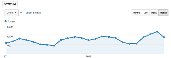
Monthly visitors 2021-22. Page views ~3 each.

My main interests in the past year have not been maths and relativity  and I have not posted here for over a year. However, the website remains fairly popular and occasionally attracts useful and nice comments especially from Petra Axolotl who was my very first mentor back in 2018. So I will continue to pay a tenner a year to keep the website going.

Happy 2023, year of the rabbit.

New Scientist Christmas Puzzle 2021

 

The grid contains 46 x 72 = 3,312 letters. Hidden inside it are the 118 elements in the periodic table, 17 known fundamental particles and 20 amino acids that make up proteins. They are revealed here. TAU and TIN occur about 15 and 31 times respectively. Two TINs come out of row 44, column 30, one going up and left, the other up and right. IRON and MUON occur three times. All other multiple occurrences are necessary if one is to have words such as ERBIUM, TERBIUM, YTTERBIUM. MUON should occur twice, the second time in MUONNEUTRINO.

View on youtube: https://youtu.be/nDXHi--u3E8

The original puzzle is here. The spreadsheet and more are here.

Powers of sine and cosine as multiple angles

I had a problem which required integrating powers of sines and cosines. 

I used integral-calculator to do the work up to a power of six. Its results are shown below. $$\fbox{$\begin{matrix}n&\int{\cos^n{\theta}d\theta}&\int{\sin^n{\theta}d\theta}\\2&\frac{\sin{\left(2\theta\right)}+2\theta}{4}&\frac{-\sin{\left(2\theta\right)}+2\theta}{4}\\3&\sin{\theta}-\frac{\sin^3{\theta}}{3}&\frac{\cos^3{\theta}}{3}-\cos{\theta}\\4&\frac{\sin{\left(4\theta\right)}+8\sin{\left(2\theta\right)}+12\theta}{32}&\frac{\sin{\left(4\theta\right)}-8\sin{\left(2\theta\right)}+12\theta}{32}\\5&\frac{\sin^5{\theta}}{5}-\frac{2\sin^3{\theta}}{3}+\sin{\theta}&-\frac{\cos^5{\theta}}{5}+\frac{2\cos^3{\theta}}{3}-\cos{\theta}\\6&\frac{\sin{\left(6\theta\right)}+9\sin{\left(4\theta\right)}+45\sin{\left(2\theta\right)}+60\theta}{192}&-\frac{\sin{\left(6\theta\right)}-9\sin{\left(4\theta\right)}+45\sin{\left(2\theta\right)}-60\theta}{192}\\\end{matrix}$}$$

There appears to be a pattern. But at the moment it is veiled. The integrals of odd powers can be found by a crafty substitution which I found here. It gives$$\int\sin^n{\theta}d\theta=\sum_{l=0}^{l=\frac{n-1}{2}}{\left(-1\right)^{l+1}B_l^{\frac{n-1}{2}}}\frac{\cos^{2l+1}{\theta}}{2l+1}+C,\ for\ odd\ n$$$$\int\cos^n{\theta}d\theta=\sum_{l=0}^{l=\frac{n-1}{2}}{\left(-1\right)^lB_l^{\frac{n-1}{2}}\frac{\sin^{2l+1}{\theta}}{2l+1}}+C,\ for\ odd\ n$$where ##B_l^n## is the binomial coefficient$$B_l^n=\frac{n!}{l!\left(n-l\right)!}$$The integrals of even powers are not so simple. I ventured into multiple angle expressions for ##\cos^n{\theta},\sin^n{\theta}## using the Chebyshev method. Multiple angles are easy integrate. I ended up with the Christmas trees at the top.

If you're interested read it here: Sine and Cosine formulas.pdf (12 pages).

3D-grapher at math3d.org

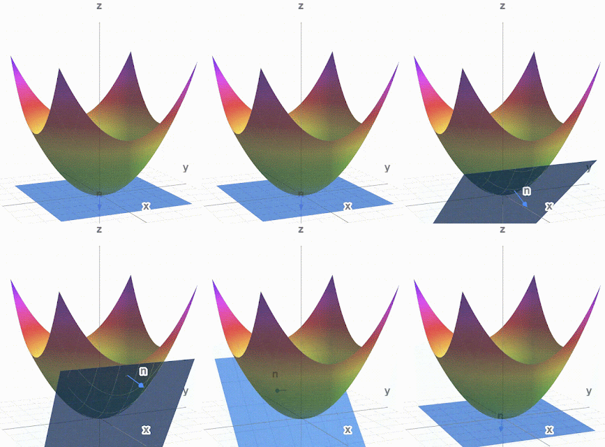
I was practicing my tensor analysis and calculated a normal vector to a surface. I wanted to see it looked orthogonal to the surface. It didn't really. So I made a tangent plane to the surface. The normal vector still looks a bit un-orthogonal but it passes all the mathematical tests.

Paraboloid, Normal vector and tangent plane ##\phi_2\left(\vec{x}\right)=\left(x^1\right)^2+\left(x^2\right)^2-x^3=0##

You can play with this at https://www.math3d.org/ybhLm7KGb and stop it from moving.

I also used Debut Video Capture to make a .avi from math3d and then cloudconvert.com to make the .gif. It is simpler than ezgif.com.

Other surfaces and vectors:

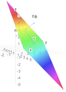
Plane and normal vectors (not v)
Play at https://www.math3d.org/fq5CtGqYa
##\phi_1\left(\vec{x}\right)=x^1+x^2+x^3=5## 

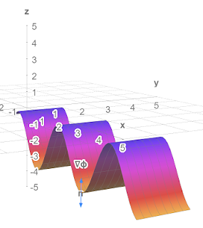
Sine wave with normal vectors
Play at https://www.math3d.org/D8xf0gZMT
##\phi_3\left(\vec{x}\right)=x^3+r_0\cos{\left(kx^1\right)}=-4## 

Lots more tools on Physics Forums at 

List of Online Calculators for Math, Physics, Earth and Other Curiosities.

Cubic equations and elliptic curves

At what ##c## does the curve change from one type to the other and what then is the leftmost point of the curve?

Answers$$c=\sqrt{\frac{32}{27}}\ \ ,\ \ x=-\sqrt{\frac{8}{3}}$$Here's why PF Challenge 2110#14.pdf (7 pages).

The Parallel Propagator and using it on the surface of a sphere

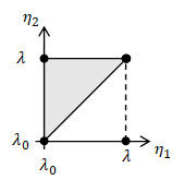
The three page Appendix I is on the parallel propagator which gives a general solution to the parallel transport equation of a vector. The appendix shows how to get this from the parallel transport equation which is, for a vector ##V^\nu## transported along a curve ##x^\mu\left(\lambda\right)## $$\frac{dx^\mu}{d\lambda}\partial_\mu V^\nu+\frac{dx^\mu}{d\lambda}\Gamma_{\mu\sigma}^\nu V^\sigma=0$$First we note that the transported vector can be calculated by$$V^\mu\left(\lambda\right)=P_{\ \ \rho}^\mu\left(\lambda,\lambda_0\right)V^\rho\left(\lambda_0\right)$$where ##V^\rho\left(\lambda_0\right)## is the vector at the start point ##x^\mu\left(\lambda_0\right)## and ##P_{\ \ \rho}^\mu\left(\lambda,\lambda_0\right)## is some matrix which is called the parallel propagator. Next we define another matrix $$A_{\ \ \rho}^\mu\left(\lambda\right)=-\Gamma_{\sigma\rho}^\mu\frac{dx^\sigma}{d\lambda}$$and then show that (dropping indices on the matrices)$$P\left(\lambda,\lambda_0\right)=I+\sum_{n=1}^{n=\infty}T_n$$where ##I## is the identity matrix and $$T_n=\int_{\lambda_0}^{\lambda}{\int_{\lambda_0}^{\eta_n}\int_{\lambda_0}^{\eta_{n-1}}{\ldots\int_{\lambda_0}^{\eta_2}A\left(\eta_n\right)A\left(\eta_{n-1}\right)\ldots A\left(\eta_1\right)}d^n\eta}$$$$=\frac{1}{n!}\int_{\lambda_0}^{\lambda}{\int_{\lambda_0}^{\lambda}\int_{\lambda_0}^{\lambda}{\ldots\int_{\lambda_0}^{\lambda}\mathcal{P}\left[A\left(\eta_n\right)A\left(\eta_{n-1}\right)\ldots A\left(\eta_1\right)\right]}d^n\eta}$$where ##\mathcal{P}## orders the matrices ##A\left(\eta_i\right)## so that ##\eta_n\geq\eta_{n-1}\geq\ldots\geq\eta_1##.

2-simplex

The first integral is over ##n##-dimensional equilateral right triangles, or ##n##-simplices and is quite hard to calculate but ##n!## ##n##-simplices make an ##n##-cube which makes the second integral which is much easier to calculate. I had a bit of trouble getting my head round all that and I tested it on a few examples including vectors transported along lines of constant latitude.  It all works!

Read about it here Commentary App I Parallel Propagator.pdf (13 pages). 

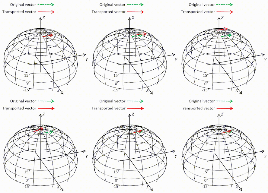
Vectors transported round latitudes calculated by parallel propagator

Note vector length never changes. ##T_n## was evaluated to 5 decimal places. 

Transport at 80°N. Vector barely
changes because it's nearly flat up there.
##T_n=0## at ##n=25##

Transport round equator. Vector remains
parallel because equator is geodesic.
##T_n=0## at ##n=1##

Transport at 15°N.
Vector rotates down by 87°.
##T_n=0## at ##n=11##

Transport at 15°S.
Vector rotates up by 87°.
##T_n=0## at ##n=11##

MTW Ex 6.2,3.1 Commutators and partial derivatives

Question

Take the mathematician's view that tangent vectors and directional derivatives are the same thing, ##u\equiv\partial_u##. Let ##u,v## be two vector fields and define their commutator in the manner familiar from quantum mechanics [not familiar to me!]$$\left[u,v\right]\equiv\left[\partial_u,\partial_v\right]\equiv\partial_u\partial_v-\partial_v\partial_u$$(a) Derive the following expression for ##\left[u,v\right]## valid in any coordinate basis$$\left[u,v\right]=\left(u^\beta v_{\ \ ,\beta}^\alpha-v^\beta u_{\ \ ,\beta}^\alpha\right)e_\alpha$$Thus despite that it looks like a second-order differential operator, ##\left[u,v\right]## is actually of first order - i.e. it is a tangent vector. 

(b) For any basis ##\left\{e_\alpha\right\}## one defines the "commutation coefficients" ##c_{\beta\gamma}^{\ \ \ \ \ \alpha}## and ##c_{\beta\gamma\alpha}## by $$\left[e_\beta,e_\gamma\right]\equiv c_{\beta\gamma}^{\ \ \ \ \ \alpha}e_\alpha;\ \ c_{\beta\gamma\alpha}=g_{\alpha\mu}c_{\beta\gamma}^{\ \ \ \ \ \mu}$$Show that ##c_{\beta\gamma}^{\ \ \ \ \ \alpha}=c_{\beta\gamma\alpha}=0## got any coordinate basis.

(c) Calculate ##c_{\hat{\beta}\hat{\gamma}}^{\ \ \ \ \ \hat{\alpha}}## for the spherical noncoordinate basis of exercise 8.1.

Answers

This was straight forward. But I learned that Hermann Schwarz outshone Euler,  Lagrange, Cauchy who were all very clever. It was Schwarz who proved that partial derivatives commute. The others didn't get it quite right apparently. So I repeated his proof and now I know when partial derivatives commute and when they don't. Hurrah.

On this exercise: 8.2 Exercise Commutators.pdf (3 pages)

On Schwarz's theorem: 8.2 Schwarz's theorem.pdf (4 pages)

And a bonus: 3.1 Exercise Components of EMF tensor.pdf (2 pages) 

MTW Ex 8.1 Practice with tensor algebra

Question

Let ##t,x,y,z## be Lorentz coordinates in flat spacetime, and let $$r=\left(x^2+y^2+z^2\right)^\frac{1}{2}\ ,\ \theta=\arccos{\left(\frac{z}{r}\right)}\ ,\ \phi=\arctan{\left(\frac{y}{x}\right)}$$be the corresponding spherical coordinates. Then$$e_0=\frac{\partial\mathcal{P}}{\partial t}\ ,\ e_r=\frac{\partial\mathcal{P}}{\partial r}\ ,\ e_\theta=\frac{\partial\mathcal{P}}{\partial\theta}\ ,\ e_\phi=\frac{\partial\mathcal{P}}{\partial\phi}$$is a coordinate basis, and $$e_{\hat{0}}=\frac{\partial\mathcal{P}}{\partial t}\ ,\ e_{\hat{r}}=\frac{\partial\mathcal{P}}{\partial r}\ ,\ e_{\hat{\theta}}=\frac{1}{r}\frac{\partial\mathcal{P}}{\partial\theta}\ ,\ e_{\hat{\phi}}=\frac{1}{r\sin{\theta}}\frac{\partial\mathcal{P}}{\partial\phi}$$is a non-coordinate basis.

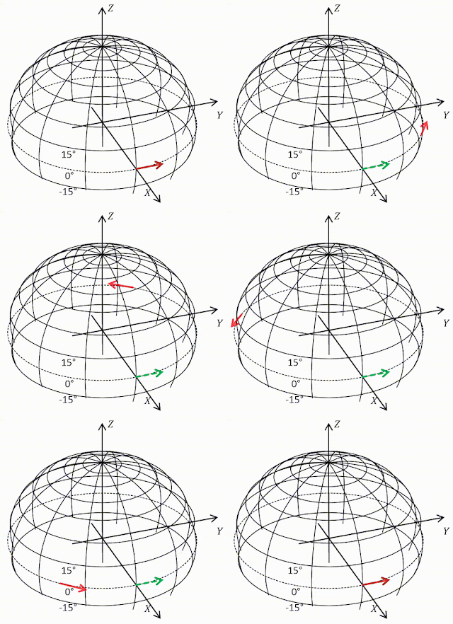
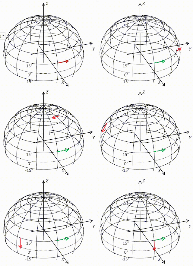
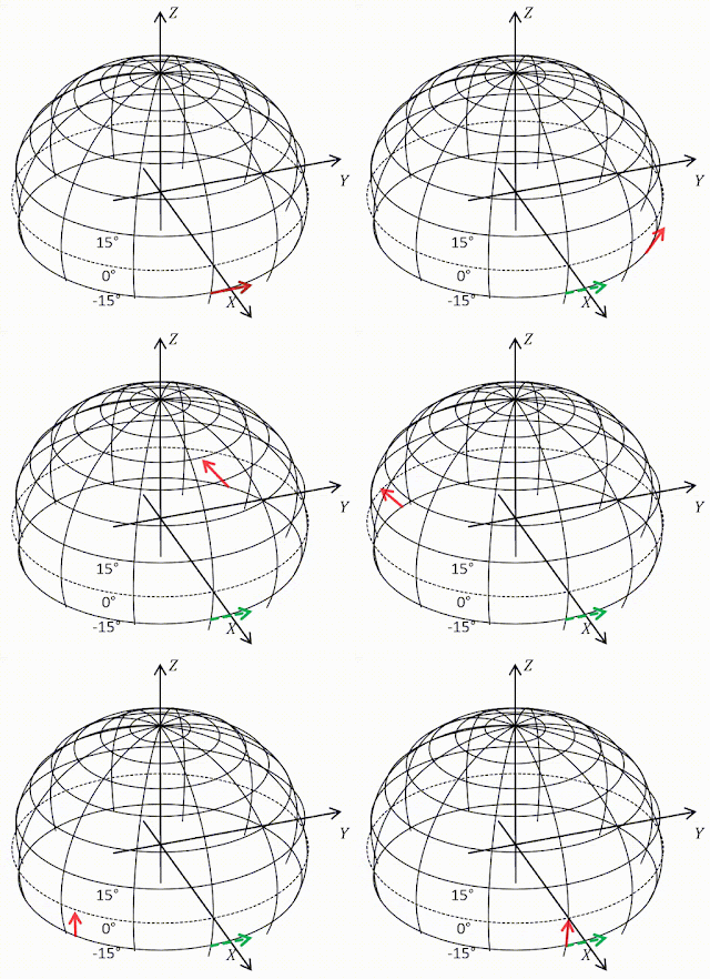
(a) Draw a picture of ##e_\theta,e_\phi,e_{\hat{\theta}},e_{\hat{\phi}}## at several different points on a sphere of constant ##t,r##.

(b) What are the one-form bases dual to these tangent-vector bases?

(c) What is the transformation matrix linking the original Lorentz frame to the spherical coordinate frame ##\left\{e_a\right\}##?

(d) Use this transformation matrix to calculate the metric components ##g_{\alpha\beta}## in the spherical coordinate basis and invert the result to get ##g^{\alpha\beta}##.

(e) Show that the non-coordinate basis ##\left\{e_{\hat{a}}\right\}## is orthonormal everywhere; i.e. that ##g_{\hat{\alpha}\hat{\beta}}=\eta_{\alpha\beta}##; i.e. that $$g=-\omega^{\hat{0}}\otimes\omega^{\hat{0}}+\omega^{\hat{r}}\otimes\omega^{\hat{r}}+\omega^{\hat{\theta}}\otimes\omega^{\hat{\theta}}+\omega^{\hat{\phi}}\otimes\omega^{\hat{\phi}}$$(f) Write the gradient of a function ##f## in terms of the spherical coordinate and noncoordinate bases.

(g) What are the components of the Levi-Civita tensor in the spherical coordinate and noncoordinate bases?

Answers

This exercise seems mainly to be concerned with putting the rules in Box 8.4 into practice. We meet a noncoordinate (anholonomic) basis. One of the features of these is that coordinates cannot be used to describe positions but you can use components to describe other tensors. So$$p^{\hat{\mu}}=\left(a,b,c,d\right)\equiv ae^{\hat{0}}+be^{\hat{r}}+ce^{\hat{\theta}}+de^{\hat{\phi}}$$is at best meaningless but$$g_{\hat{\alpha}\hat{\beta}}=\left(\begin{matrix}a&0&0&0\\0&b&0&0\\0&0&c&0\\0&0&0&d\\\end{matrix}\right)$$is valid and is the answer to (d) when ##a=-1,b=c=d=1## .

I found an excellent new way of  creating animated gifs. Which I used for the answer to (a) below. The diagrams for ##e_{\hat{\theta}},e_{\hat{\phi}}## are a good indication of (e).

Coordinate bases going round equator	Coordinate bases going over pole
Non-coordinate bases going round equator	Non-coordinate bases going round equator

Full details at 8.1 Exercise Practise with Tensor Algebra.pdf (12 pages).

MTW Ex 8.5 A sheet of paper in polar coordinates

Question

The two-dimensional metric for a flat sheet of paper in polar coordinates is ##\left(r,\theta\right)## is$${ds}^2={dr}^2+r^2{d\phi}^2$$or in modern notation$$\mathbf{g}=\mathbf{d}r\otimes\mathbf{d}r+r^2\mathbf{d}\phi\otimes\mathbf{d}\phi$$Presumably the coordinates are ##\left(r,\phi\right)## not ##\left(r,\theta\right)##.

(a) Calculate the connection coefficients using 8.24.

(b) Write down the geodesic equation in ##\left(r,\phi\right)## coordinates.

(c) Solve these equations for ##r\left(\lambda\right)## and ##\phi\left(\lambda\right)## and show that the solution is a uniformly parameterized straight line. (##x\equiv r\cos{\phi}=a\lambda+b## for some ##a## and ##b##, ##y\equiv r\sin{\phi}=j\lambda+k## for some ##j## and ##k##).

(d) Verify that the noncoordinate basis ##\mathbf{e}_{\hat{r}}\equiv\mathbf{e}_r=\frac{\partial\mathcal{P}}{\partial r},\ \mathbf{e}_{\hat{\phi}}\equiv r^{-1}\mathbf{e}_\phi=r^{-1}\frac{\partial\mathcal{P}}{\partial\phi},\ \ \mathbf{\omega}^r=\mathbf{d}r,\ \mathbf{\omega}^{\hat{\phi}}=r\mathbf{d}\phi## is orthonormal, and that ##\left<\mathbf{\omega}^\alpha,\mathbf{e}_{\hat{\beta}}\right>=\delta_{\ \ \hat{\beta}}^{\hat{\alpha}}##. Then calculate the connection coefficients of this basis from a knowledge [part (a)] of the connection of the coordinate basis.

Answer

I think 1) there are hats missing from omega indices and 2) 'modern notation' might not be very modern. I find it surprising that such an old, respected book has so many misprints.

a,b,c were straightforward. (d) contained the surprises. The ##\left(\hat{r},\hat{\phi}\right)## system (as we might call it) was orthonormal. The ##\left(r,\phi\right)## system was not, it was only orthogonal. The connection coefficients of the ##\left(\hat{r},\hat{\phi}\right)## system are not all symmetric in the lower two indices: ##\Gamma_{\hat{\phi}\hat{r}}^{\hat{\phi}}=0\neq\Gamma_{\hat{r}\hat{\phi}}^{\hat{\phi}}=\frac{1}{r}## which we prove. The method of calculating the coefficients is a great exercise in the piercing counter ##\left<,\right>##. 

##{\hat{e}}_r,{\hat{e}}_\phi## form a noncoordinate basis because, if we use them, the same point can have different coordinates. We show that is true. ##e_r,e_\phi## do not suffer from this problem.

Additionally we calculate the commutators (or Lie derivatives) ##\left[e_r,e_\phi\right]=\left[\partial_r,\partial_\phi\right]## and ##\left[{\hat{e}}_r,{\hat{e}}_\phi\right]##. The first vanishes the second does not. This is a proof that the first is a coordinate (holonomic) basis and the second a noncoordinate (anholonomic) basis where you can't use coordinates. So you can't say ##\left[{\hat{e}}_r,{\hat{e}}_\phi\right]=\left[\partial_{\hat{r}},\partial_{\hat{\phi}}\right]##. even though you can use the indices as in ##\Gamma_{\hat{\phi}\hat{r}}^{\hat{\phi}}=0##.

Tiptoe through noncoordinate minefield at 8.5 Exercise Plane polar coordinates.pdf  (14 pages)

Pythagoras's and Newton's formulas for 𝝅

This fun video by Veritasium gives the story of Pythagoras and Newton and ##\pi## but it doesn't go into details. I wanted to know more.

Pythagoras calculated ##\pi## by placing regular n-agons just inside and outside a unit circle and calculating their perimeters. Some examples are shown below.

Apparently he stopped at a 96-agon. I reckon the result he got was$$48\sqrt{2-2\sqrt{\frac{1}{2}+\frac{1}{2}\sqrt{\frac{1}{2}+\frac{1}{4}\sqrt{2+\sqrt3}}}}<\pi<\frac{96\sqrt{2-2\sqrt{\frac{1}{2}+\frac{1}{2}\sqrt{\frac{1}{2}+\frac{1}{4}\sqrt{2+\sqrt3}}}}}{\sqrt{2+2\sqrt{\frac{1}{2}+\frac{1}{2}\sqrt{\frac{1}{2}+\frac{1}{4}\sqrt{2+\sqrt3}}}}}$$It was accurate to four significant digits and not surprisingly he stopped! He didn't even have decimal numbers.

The second last person to use this method in anger was Ludolph van Ceulen in about 1600 who did a ##2^{62}##-agon and still only got 35 decimal places. Apparently it took him 25 years. Nutter.

Then along came Newton (about 1700) and he used calculus (which he had just invented) and the binomial theorem to get$$\pi\approx-\frac{3\sqrt3}{2}+6-\left(\frac{1}{4}+\frac{3}{320}+\frac{45}{53,760}+\frac{1,575}{22,855,680}\right)$$That's accurate to five significant digits and a good deal easier to calculate. The further you go the better it gets:

Here's how they did it Newtons formula for pi.pdf (10 pages).

Kinetic Energy ≠ ½mv²

While studying ##E=mc^2## I keep noticing that kinetic energy is not ##\frac{1}{2}mv^2## as we were always taught in school. The relativistic formula is, in various forms, $$K_{rel}=\frac{c^3}{\sqrt{c^2-v^2}}-c^2=c^2\left(\frac{1}{\sqrt{1-\beta^2}}-1\right)=c^2\left(\frac{1}{2}\beta^2+\frac{3}{8}\beta^4+\ldots\right)$$where ##\beta=v/c##.

On May 2nd 2021 the Parker Solar Probe achieved a velocity of 532,000 km/h which is about ##0.0005c##. That gives

\begin{align}\frac{K_{rel}}{c^2}=1.25000023\times{10}^{-7}\ ,\ \frac{K_{cl}}{c^2}=1.25\times{10}^{-7}&\phantom {10000}(8)\nonumber\end{align}Not much difference. The mass of the probe is about 600kg so the difference is ##2.3\times{10}^3\ Joules## which might keep a phone going for an hour.

 

The difference is more noticeable at much higher velocities. At ##0.1c## the difference is about 1%. It goes wild as you approach the speed of light.

A bit more here: 2.2 Kinetic energy.pdf (1 page)

Why does E=mc²?

Trying to follow the second worked example in Box 2.2 of Misner, Thorne, Wheeler I realised that I did not know how Einstein proved ##E=mc^2## and, when I checked in my books, both MWT and Carroll gloss it over! Using Einstein's 1905 paper, an internet video and the relativistic Doppler shift formulas given by Wikipedia I now do. Here's my version based on those.

We take two scenarios 

1) observe the object, in its rest frame, emitting two pulses of light with energy ##E/2## in opposite directions so that it does not change velocity and then we take off in a rocket with velocity ##v## so the object has some kinetic energy ##K_1## 

2) measure its kinetic energy ##K_2## from a frame moving with velocity ##v## then it emits the light which will have energy doppler shifted according to $$E_r=E\left(1+\frac{v^2}{2c^2}\right)$$After the emission we are now in the final state of scenario 1 and the object must have kinetic energy ##K_1## and total energy ##K_1-E##.

In both scenarios the object lost energy by radiation and gained kinetic energy (because the observer started moving) and we end up at the same place. The total energy must be the same in either scenario therefore$$K_1-E=K_2-E\left(1+\frac{v^2}{2c^2}\right)\Rightarrow\frac{Ev^2}{2c^2}=K_2-K_1$$We know how to calculate the kinetic energy (##mv^2/2##) and the velocities of the kinetic energies are the same so the masses must have changed. So$$\frac{Ev^2}{2c^2}=m_2\frac{v^2}{2}-m_1\frac{v^2}{2}\Rightarrow E=\Delta Mc^2$$where ##\Delta M## is the change in the mass of the object. Furthermore we conclude that if one could get all the energy out of an object of mass ##m## that energy would be

$$E=mc^2$$For more details including the derivation of ##E_r## see the very short 2.2 Box E=mc2.pdf.

Coming soon. More on that Box 2.2.

2.5 Differential forms

Vector ##U## (solid) and
1-form ##\widetilde{U}## (dashed)

In section 2.5 of Misner, Thorne, Wheeler 'differential forms' or '1-forms' are introduced and there is soon a fairly elaborate recipe for constructing 1-forms ##\widetilde{U}## from a vector ##U##. I reproduce it below. I tried out the recipe on some of the sample vectors shown and it seemed to work. A one form ##\widetilde{U}## is shown as a set of planes, whose spacing is defined, and which have a positive sense, or direction, as shown by a dashed arrow (which is not a vector). It would seem that you could equally well show the 1-form by a dashed arrow perpendicular (in the Euclidean sense) to the planes whose direction and length would show the positive sense and the spacing of the planes of ##\widetilde{U}##. You can. And I implemented it in a spreadsheet and made the amusing gif on the right. Then I saw the joke.

The recipe

Figure 2.7. Several vectors, ##A,B,C,D,E##, and corresponding 1-forms ##\widetilde{A},\widetilde{B},\widetilde{C},\widetilde{D},\widetilde{E}##. The process of drawing ##\widetilde{U}## corresponding to a given vector ##U## is quite simple. 1) Orient the surfaces of ##\widetilde{U}## orthogonal to the vector ##U## . (Why? Because any vector ##V## that is perpendicular to ##U## must pierce no surfaces of ##\widetilde{U}## (##0=U\bullet V=U,V##) and must therefore lie in a surface of ##\widetilde{U}##.) 2) Space the surfaces of  ##\widetilde{U}## so the number of surfaces pierced by some arbitrary vector ##Y## (e.g., ##Y=U##) is equal to ##Y\bullet U##.

Note that in the figure the surfaces of ##\widetilde{B}## are, indeed, orthogonal to ##B##; those of ##\widetilde{C}## are, indeed, orthogonal to ##C##, etc. If they do not look so, that is because the reader is attributing Euclidean geometry, not Lorentz geometry, to the spacetime diagram. He should recall, for example, that because ##C## is a null vector, it is orthogonal to itself (##C\bullet C=0##), so it must itself lie in a surface of the 1-form  ##\widetilde{C}##. Confused readers may review spacetime diagrams in a more elementary text, e.g., Taylor and Wheeler (1966)."

Read it here, including punchline: 2.5 Differential forms.pdf. (6 pages)

Wave packets

I have started to read Misner, Thorne and Wheeler's great tome on gravitation. It starts quite differently from Carroll by emphasizing a coordinate free view. (Pythagoras and Euclid proved a lot without coordinates which were popularized René Descartes about 2000 years after them.) In section 2.5 MTW claim that the pattern of surfaces (named ##\widetilde{{k}}##) generated by a matter wave (aka De Broglie wave) provide the simplest example of 1-forms which we know are covariant vectors or vectors with indices downstairs. I need to revise my quantum mechanics and find a book on the internet by JD Cresser. I think it is a bit hand-wavey but it helps me understand a bit more. The first step is generating a wave packet from a regular sine wave (or similar). The wave packet will be a particle.

Cresser starts with a cosine wave with a wave number 5 so the equation is ##\psi=\cos{5x}##. In this case the wave number is the number of waves that fit in a length ##2\pi##. Sometimes it is then number per unit length. He then takes another wave with wave number 5.5. The '2 sine waves' image shows them both. You can see a patter emerging. That becomes clearer if you add them and divide by 2 as shown in '2 waves added'. It is the famous beat that is heard if two nearby notes are played at the same time. He then adds more, all with wave numbers in the range 4.75 to 5.25 and claims that by adding even more you will get a wave packet. That is not true! If you add in more and more waves the picture remains the same, there are always small bulges and the large bulges just move off into the remote distance. The range shown is for ##x=\pm65##. On the 9 wave picture there are large bulges at about ##x=\pm100,\pm200\ldots## and on the 17 wave picture at about ##x=\pm200,\pm400\ldots## (I checked three of those). Then something in his text suggested that I should add waves in a larger range and that does produce a wonderful wave packet.

With 999 waves and ##k## in the range 4 to 6 the picture improves and with a slightly larger range, 0 to 10, it is a pretty decent wave packet (although I think there might be another spike well off the chart - try it yourself!).

Numbers and wave generator at Wave packets.pdf (4 pages) 

Cosmic distance measures

 I am still trying to prove the relationships between different cosmic distance measures$$d_L=\left(1+z\right)d_M=\left(1+z\right)^2d_A$$and I'm sill not there. on the way I came across a nice graph on Wikipedia comparing them for various ##z## and wondered if I could reproduce it. My version and the Wikipedia one are shown below, I was pleased.

Spot the difference

Here's how and my first attempts at proving that formula: Commentary 8.5.4 More distances.pdf (10 pages)

Three years old

The very first post on this blog was on Thursday, 15 March 2018. So we're over three years old and now getting nearly 3,000 pageviews per month. There was a mysterious big uptick in September last year. 

adpushup.com says that I might get $70 per year from adverts. google.com/adsense says 5,000€. Dreaming.

Thanks to all you readers!

Luminosity distance

In section 8.5 we are looking at redshifts and distances. We started in an FLRW universe with metric

\begin{align}{ds}^2=-{dt}^2+a^2\left(t\right)\left[\frac{{\rm dr}^2}{1-\kappa r^2}+r^2{d\theta}^2+r^2\sin^2{\theta}{d\phi}^2\right]&\phantom {10000}(1)\nonumber\end{align}or

\begin{align}{ds}^2=-{dt}^2+a^2\left(t\right){R_0}^2\left[{d\chi}^2+{S_k}^2\left(\chi\right){d\Omega}^2\right]&\phantom {10000}(2)\nonumber\end{align}where ##k\in\left\{-1,0,1\right\}## and

\begin{align}S_k\left(\chi\right)\ \equiv\left\{\begin{matrix}\sin{\chi},&k=+1&\rm{closed}\\\chi,&k=0&\rm{flat}\\\sinh{\chi}&k=-1&\rm{open}\\\end{matrix}\right.&\phantom {10000}(3)\nonumber\end{align}(2) is Carroll's 8.106, a sort of hybrid FLRW metric.

This starts at Carroll's 8.110 where he defines distance luminosity ##d_L## which you can get if you know the absolute luminosity of a star (or galaxy) and can measure the amount of light that reaches you. We then correct that for the expansion of the universe and further correct it because the universe deviates from a perfect sphere according to ##S_k\left(\chi\right)##. We arrive at the celebrated and complicated formula at (4) which uses (5) which uses (6) .

\begin{align}d_L=\left(1+z\right)\frac{{H_0}^{-1}}{\sqrt{\left|\Omega_{c0}\right|}}S_k\left[\sqrt{\left|\Omega_{c0}\right|}\int_{0}^{z}\frac{dz^\prime}{E\left(z^\prime\right)}\right]&\phantom {10000}(4)\nonumber\end{align}where

\begin{align}E\left(z\right)=\left[\sum_{i(c)}{\Omega_{i0}\left(1+z\right)^{n_i}}\right]^\frac{1}{2}&\phantom {10000}(5)\nonumber\end{align}and there are four elements in the summation, one each for matter, radiation, curvature and vacuum energy density. ##\Omega_i## is the density parameter which we met before and was defined as 

\begin{align}\Omega_i=\frac{8\pi G}{3H^2}\rho_i&\phantom {10000}(6)\nonumber\end{align}where the ##\rho_i## are the energy densities for each of those four things. ##\Omega_i## and ##H##, the Hubble factor acquire a 0 subscript for their values in the present epoch. 

I then try to calculate (4) from known values. ##\Omega_{c0}## the pseudo-density parameter for curvature comes from Friedmann's equation and the other three density parameters. That radiation energy is negligible, matter energy density corresponds to what is usually called ordinary (baryonic) plus dark matter and vacuum energy density is dark energy. The integral in (4) must be calculated numerically and I plotted below (page 10 in the pdf). After that we have plots of luminosity distance vs redshift for the three kinds of universe determined by ##k## in (3). Luminosity distances greater 100 billion light years are quite easy to get. I thought everything was a failure until I found some distance calculators which gave more or less the same! According to Carroll, these distances are compared with those measured from absolute and apparent luminosity. Luminosity distance is mighty peculiar. Coming soon: Proper motion distance and Angular diameter distance.

I also found that there is a missing divide by sign in Carroll's equation 8.122.

Read all about it at Commentary 8.5.2 Redshifts and Distances.pdf (12 pages)

Exercise 1.9 Energy momentum tensor of point particles

Question

Point particles in proton

For a system of discrete point particles the energy-momentum tensor takes the form$$
T_{\mu\nu}=\sum_{a}{\frac{p_\mu^{\left(a\right)}p_\nu^{\left(a\right)}}{p^{0\left(a\right)}}\delta^{\left(3\right)}\left(\mathbf{x}-\mathbf{x}^{\left(a\right)}\right)}
$$where the index ##a## labels the different particles. Show that, for a dense collection of particles with isotropically distributed velocities, we can smooth over the individual particle worldlines to obtain the perfect-fluid energy-momentum tensor 1.114. 

1.114 was$$
\mathbf{T}^{\mu\nu}=\left(\rho+p\right)U^\mu U^\nu+p\eta^{\mu\nu}
$$where ##\rho## is the energy density of the fluid measured in its rest frame (rest-frame energy density) and ##p## is the isotropic rest-frame pressure. ##T^{\mu\nu}## is the energy-momentum tensor of a fluid element with a four velocity ##U^\mu##. 

Answer

Carroll is setting plenty of traps here. 

• The ##p##'s in second equation are rest-frame pressure and the ##p##'s in the first are 4-momentum components.
• What does ##\delta^{\left(3\right)}\left(\mathbf{x}-\mathbf{x}^{\left(a\right)}\right)## mean? Carroll gives no hint.
• How do you smooth over the individual particle worldlines?
• Having indices down on the first equation is just perverse. Raise them immediately! 
• There is a conceptual problem. The first equation concerns a point particle and the second concerns a particle of fluid which contains lots of point particles. I try to call the fluid particle a fluid element. It's a bit weird. We are doing summations over the point particles and we will be integrating and differentiating over fluid elements which are bigger but nevertheless still small enough to be treated as points in our calculus.

First I found out what ##\delta^{\left(3\right)}\left(\mathbf{x}-\mathbf{x}^{\left(a\right)}\right)## is and justified the expression for the energy-momentum of the point particle. I then got stuck until I found a solution by Alexey Bobrick on physics.stackexchange. It starts well but ends not so well, I believe. I think I did a little better.

Read here: Ex 1.09 Energy momentum tensor of point particles.pdf (6 pages)

Super Nova

Kepler's Supernova* remnant in background

There is a unified catalogue of 5526 supernova (SN) by D. Lennarz et al and I want to extract the Type Ia Super Novae along with their magnitudes, redshifts and distances to see how those compare with what I have been learning out about redshifts and luminosity and other distances in section 8.3. Type Ia Super Nova are all supposed to have the same absolute magnitude of −19.3 (about 5 billion times brighter than the Sun). I was able to confirm Hubble's law and learnt that that the mighty peculiar formula for Type Ia Supernova: ##m=5\log_{10}{D}-24.3## for the fall off in apparent magnitude ##m## with distance ##D## is in fact an inverse power law. And that corrections for the expansion and curvature of the universe at this range (about a fifteenth of the size of the visible universe) are immaterial. 

Read all about it at Commentary 8.5.3 Super Nova.pdf (4 pages)

* Kepler's supernova was the last one ever seen in the Milky Way. That was 1604. It would be exciting if there was another one soon. (But not too close!)